
Setup
Google Colab
Click the badge above to open this notebook in Colab. The notebook installs or activates dependencies in the setup cells below.
Local installation
Run the following from the repository root before opening this notebook locally:
python -m pip install matplotlib numpy scipyThe notebook uses bundled Graver data by default; optional 4ti2 tooling is only needed when regenerating bases.
Learning objectives
By the end of this notebook you will be able to:
Explain how Graver-basis directions can augment feasible integer solutions.
Run the GAMA workflow on a nonlinear integer programming instance with bundled or computed Graver data.
Compare complete and sampled Graver bases across objective improvement, iterations, and runtime.
Interpret the speed-quality tradeoff between exact augmentation data and smaller sampled direction sets.
Prerequisites
Mathematical background: Integer programming, feasible sets, nonlinear objective functions, and basic runtime comparisons.
Prior notebooks: Notebook 2 (QUBO) and the binary/integer modeling ideas from Notebook 1.
Accounts required: None; optional Py4ti2int32 or 4ti2 support can compute Graver bases instead of using bundled data.
Python version: Python 3.9+ with NumPy, Matplotlib, and the repository’s GAMA dependencies.
Environment and execution notes
For local execution from the repository root, run uv sync --group qubo before launching Jupyter so the Python scientific stack used below is available. If Py4ti2int32 is installed, the notebook computes the Graver basis directly; otherwise it falls back to the bundled graver.npy file so the rest of the workflow still runs.
In Google Colab, the notebook reuses the bundled graver.npy file whenever Py4ti2int32 is unavailable, which keeps the student-facing workflow focused on the GAMA steps rather than on an external 4ti2 installation.
Introduction to GAMA
The Graver Augmentation Multiseed Algorithm (GAMA) was proposed by Alghassi, Dridi, and Tayur in the works listed in Reference [1] and Reference [2]. The three main ingredients of this algorithm, designed to solve integer programs with linear constraints and nonlinear objective, are:
Computing the Graver basis (or a subset of it) of an integer program.
Performing an augmentation.
Initializing the algorithm from several points because Graver augmentation is guaranteed to find a global optimum only for certain objective functions.
This algorithm can be adapted to take advantage of Quantum Computers by leveraging them as black-box Ising/QUBO problem solvers. In particular, obtaining several feasible solution points for the augmentation and computing the kernel of the constraint matrix can be posed as QUBO problems. After obtaining these solutions, other routines implemented in classical computers are used to solve the optimization problems, making this a hybrid quantum-classical algorithm.
Introduction to Graver basis computation
This notebook makes simple computations of Graver basis. Because of the complexity of these computations, we suggest that for more complicated problems you install the excellent 4ti2 software, an open-source implementation of several routines useful for the study of integer programming through algebraic geometry. It can be used as a stand-alone library and called from C++ or from Python. In Python, there are two ways of accessing it, either through Sage or by compiling 4ti2 directly and installing a Python wrapper.
A Graver basis is defined as
where are the minimal Hilbert basis of in each orthant.
Equivalently we can define the Graver basis as the -minimal set of a lattice
where the partial ordering holds whenever and for all .
Here we do not interact with quantum hardware. Instead, we obtain a problem’s Graver basis with 4ti2 and study how the search behaves when only a subset of that basis is available.
try:
  import google.colab
  IN_COLAB = True
except Exception:
  IN_COLAB = False

try:
  if not IN_COLAB:
    from Py4ti2int32 import graver as py4ti2_graver
    HAS_PY4TI2 = True
  else:
    py4ti2_graver = None
    HAS_PY4TI2 = False
except ImportError:
  py4ti2_graver = None
  HAS_PY4TI2 = False
from pathlib import Path
from urllib.request import urlretrieve

import matplotlib.pyplot as plt
import numpy as np
from typing import Callable
import itertools
import random
import time
Problem statement
By default, the GAMA computation below uses Example 4 from the code, which corresponds to Case 2 in the original GAMA paper. The problem is derived from finance and deals with the maximization of expected returns on investments and the minimization of the variance.
This particular instance of convex INLP has , , , and . The matrix is a matrix with 1’s and 0’s and the vector is half of the sum of the rows of , in this case .
To make this Example 4 run reproducible, the notebook loads one fixed realization of the coefficient vectors from notebooks_data/3-GAMA_example4_coefficients.csv, reuses precomputed feasible starts from notebooks_data/3-GAMA_example4_feasible_starts.csv, and traverses a deterministic Graver-direction permutation. The remaining GAMA method below uses this saved Example 4 instance: complete-basis greedy augmentation, a 10-direction partial-basis greedy augmentation, and several larger fractions of the basis.
The Graver basis of this matrix has 29789 elements, which on a standard laptop using 4ti2 takes about 5 seconds to compute. When Py4ti2int32 is available, the notebook computes it directly; otherwise it reuses the bundled graver.npy file.
Class examples
The original GAMA class notebook used EXAMPLE = 1, EXAMPLE = 2, EXAMPLE = 3, and EXAMPLE = 4. Examples 1-3 are retained here as class-reference problem definitions. By default, the executable GAMA workflow below continues with the saved Example 4 portfolio instance.
Example 1: illustrative Graver augmentation
This example uses
The variable bounds are . In the original class notebook, the objective is to minimize distance to 5.
Example 2: four-variable linear example
This example uses
The variable bounds are .
Example 3: alternate four-variable linear example
This example uses
The variable bounds are .
Example 4: saved portfolio instance
Let
This particular instance of convex INLP has , , , , . and each is half the sum of the -th row of . In this example, .
The remaining GAMA method below uses this saved Example 4 instance: complete-basis greedy augmentation, a 10-direction partial-basis greedy augmentation, and several larger fractions of the basis.
First we would write this problem as an unconstrained one by penalizing the linear constraints as quadratics in the objective. Let’s first define the problem parameters.
To switch among the class examples, change SELECTED_GAMA_EXAMPLE in the next code cell to 1, 2, 3, or 4, then rerun the notebook from that cell downward. Example 4 remains the default because it is the saved portfolio instance used for the executed results below.
SELECTED_GAMA_EXAMPLE = 4  # Change to 1, 2, 3, or 4, then rerun from this cell downward.


def load_gama_example(example_id: int) -> dict[str, object]:
    """Return one of the class-reference GAMA examples."""
    if example_id == 1:
        return {
            "name": "Example 1: illustrative Graver augmentation",
            "A": np.array([[1, 1, 1, 1], [1, 5, 10, 25]], dtype=int),
            "b": np.array([[21], [156]], dtype=int),
            "x0": np.array([1, 15, 3, 2], dtype=int),
            "x_lo": np.zeros(4, dtype=int),
            "x_up": 15 * np.ones(4, dtype=int),
            "c": None,
            "objective": "distance_to_5",
            "graver_directions": np.array(
                [
                    [5, -6, 0, 1],
                    [5, -9, 4, 0],
                    [0, 3, -4, 1],
                    [5, -3, -4, 2],
                    [5, 0, -8, 3],
                ],
                dtype=int,
            ),
        }
    if example_id == 2:
        return {
            "name": "Example 2: four-variable linear example",
            "A": np.array([[1, 1, 1, 1], [1, 2, 3, 4]], dtype=int),
            "b": np.array([[10], [21]], dtype=int),
            "x0": np.array([1, 8, 0, 1], dtype=int),
            "x_lo": np.zeros(4, dtype=int),
            "x_up": 21 * np.ones(4, dtype=int),
            "c": np.array([0, 1, 0, 2], dtype=int),
            "objective": "linear",
            "graver_directions": np.array(
                [
                    [1, -2, 1, 0],
                    [2, -3, 0, 1],
                    [1, -1, -1, 1],
                    [0, 1, -2, 1],
                    [1, 0, -3, 2],
                ],
                dtype=int,
            ),
        }
    if example_id == 3:
        return {
            "name": "Example 3: alternate four-variable linear example",
            "A": np.array([[1, 1, 1, 1], [0, 1, 2, 3]], dtype=int),
            "b": np.array([[10], [15]], dtype=int),
            "x0": np.array([3, 0, 6, 1], dtype=int),
            "x_lo": np.zeros(4, dtype=int),
            "x_up": 10 * np.ones(4, dtype=int),
            "c": np.array([1, 3, 14, 17], dtype=int),
            "objective": "linear",
            "graver_directions": np.array(
                [
                    [2, -3, 0, 1],
                    [1, -2, 1, 0],
                    [1, -1, -1, 1],
                    [0, 1, -2, 1],
                    [1, 0, -3, 2],
                ],
                dtype=int,
            ),
        }
    if example_id == 4:
        return {
            "name": "Example 4: saved portfolio instance",
            "A": np.array(
                [
                    [1, 1, 1, 1, 1, 1, 1, 1, 1, 1, 0, 1, 0, 1, 0, 1, 0, 1, 1, 1, 0, 1, 0, 1, 0],
                    [1, 1, 1, 1, 0, 1, 0, 1, 0, 0, 1, 0, 0, 0, 1, 0, 0, 1, 0, 1, 1, 1, 1, 1, 1],
                    [0, 1, 0, 0, 0, 1, 0, 1, 0, 1, 1, 0, 1, 1, 0, 1, 1, 0, 0, 1, 0, 0, 1, 1, 1],
                    [0, 0, 0, 0, 0, 0, 0, 1, 0, 1, 1, 1, 0, 1, 1, 1, 1, 0, 0, 1, 0, 0, 0, 0, 0],
                    [0, 1, 1, 1, 1, 1, 0, 0, 0, 1, 0, 0, 0, 1, 0, 0, 0, 0, 0, 1, 0, 1, 0, 1, 0],
                ],
                dtype=int,
            ),
            "b": np.array([[9], [8], [7], [5], [5]], dtype=int),
            "x0": np.array([1, 1, 1, 1, -1, 1, 1, 1, 1, 1, 1, 1, -2, 1, 0, -1, 0, 1, -1, 1, -2, -2, 1, 1, 1], dtype=int),
            "x_lo": None,
            "x_up": None,
            "c": None,
            "objective": "portfolio",
            "graver_directions": None,
        }
    raise ValueError(f"Unknown GAMA example {example_id}; choose 1, 2, 3, or 4.")


example_data = load_gama_example(SELECTED_GAMA_EXAMPLE)
A = example_data["A"]
b = example_data["b"]
x0 = example_data["x0"]
x_lo = example_data["x_lo"] if example_data["x_lo"] is not None else -2 * np.ones_like(x0)
x_up = example_data["x_up"] if example_data["x_up"] is not None else 2 * np.ones_like(x0)
c = example_data["c"]
m, n = A.shape

print(f"Running {example_data['name']} with A shape {A.shape} and {len(x0)} variables.")


def resolve_example_data_path(filename: str) -> Path | None:
    """Return the path to a shared Notebook 3 data file when it exists."""
    candidates = [
        Path("notebooks_data") / filename,
        Path("..") / "notebooks_data" / filename,
        Path("/content/QUBONotebooks/notebooks_data") / filename,
        Path("/content/notebooks_data") / filename,
    ]
    for candidate in candidates:
        if candidate.exists():
            return candidate
    return None


def load_shared_csv(filename: str, dtype=float) -> np.ndarray | None:
    """Load a shared Notebook 3 CSV asset when it is available."""
    data_path = resolve_example_data_path(filename)
    if data_path is None:
        return None
    return np.loadtxt(data_path, delimiter=",", dtype=dtype)


def load_shared_coefficients(num_variables: int) -> tuple[np.ndarray, np.ndarray]:
    """Return the fixed `mu` and `sigma` vectors shared by both notebooks.

    Returns
    -------
    tuple[np.ndarray, np.ndarray]
        The expected-return vector `mu` and the volatility vector `sigma`.
    """
    coeffs = load_shared_csv("3-GAMA_example4_coefficients.csv", dtype=float)
    if coeffs is None:
        rng = np.random.default_rng(1729)
        mu = rng.random(num_variables)
        sigma = rng.random(num_variables) * mu
        print("Shared coefficient file not found; generating deterministic coefficients with seed 1729.")
        return mu, sigma

    coeffs = np.atleast_2d(coeffs)
    if coeffs.shape != (2, num_variables):
        raise ValueError(f"Expected coefficient array with shape (2, {num_variables}), found {coeffs.shape}.")
    return coeffs[0], coeffs[1]


# Parameters of objective function
epsilon = 0.01
if SELECTED_GAMA_EXAMPLE == 4:
    mu, sigma = load_shared_coefficients(n)
else:
    mu = np.zeros(n, dtype=float)
    sigma = np.zeros(n, dtype=float)


def load_precomputed_graver_basis() -> np.ndarray:
    """Load the bundled Graver basis from the repository or the Colab workspace."""
    candidates = [
        Path("notebooks_py") / "graver.npy",
        Path("graver.npy"),
        Path("/content/graver.npy"),
        Path("/content/QUBONotebooks/notebooks_py/graver.npy"),
    ]
    for candidate in candidates:
        if candidate.exists():
            return np.array(np.load(candidate))

    download_path = Path("/content/graver.npy")
    download_path.parent.mkdir(parents=True, exist_ok=True)
    urlretrieve(
        "https://github.com/JuliaQUBO/QUBONotebooks/raw/main/notebooks_py/graver.npy",
        download_path,
    )
    return np.array(np.load(download_path))


def graver_basis_for_selected_example() -> np.ndarray:
    """Return built-in Graver directions for small examples or the Example 4 basis."""
    if example_data["graver_directions"] is not None:
        directions = np.array(example_data["graver_directions"], dtype=int)
        print(f"Using {len(directions)} built-in Graver directions for Example {SELECTED_GAMA_EXAMPLE}.")
        return directions

    if HAS_PY4TI2:
        start = time.process_time()
        directions = py4ti2_graver("mat", A.tolist())
        print(time.process_time() - start, "seconds to compute Graver basis")
        return np.array(directions, dtype=int)

    if not IN_COLAB:
        print("Py4ti2int32 is not available locally; loading the bundled graver.npy instead.")
    else:
        print("The Graver basis has 29789 elements in this case.")
    return np.array(load_precomputed_graver_basis(), dtype=int)


r = graver_basis_for_selected_example()
Running Example 4: saved portfolio instance with A shape (5, 25) and 25 variables.
Py4ti2int32 is not available locally; loading the bundled graver.npy instead.
# Objective function definition
def f(x):
    """Evaluate the selected example objective for a candidate point `x`."""
    x = np.asarray(x)
    if SELECTED_GAMA_EXAMPLE == 1:
        return np.sum(np.abs(x - 5))
    if SELECTED_GAMA_EXAMPLE == 4:
        return -np.dot(mu, x) + np.sqrt(((1 - epsilon) / epsilon) * np.dot(sigma**2, x**2))
    return np.dot(c, x)


# Constraints definition
def const(x):
    """Return True when `x` satisfies the linear constraints `A x = b`."""
    return np.array_equal(np.asarray(A @ np.asarray(x)).reshape(-1), np.asarray(b).reshape(-1))
# Define rules to choose augmentation element, either the best one (argmin) or the first one that is found
def argmin(iterable):
    """Return the index and value of the best augmentation candidate."""
    return min(enumerate(iterable), key=lambda x: x[1])

def greedy(iterable):
    """Return the first improving augmentation candidate, or the last one if none improve."""
    found_candidate = False
    for i, val in enumerate(iterable):
        found_candidate = True
        if val[1] != 0:
            return i, val
    if not found_candidate:
        raise ValueError("greedy() called with empty candidate set")
    return i, val
# Bisection rules for finding best step size
def bisection(g: np.ndarray, fun: Callable, x: np.ndarray, x_lo: np.ndarray = None, x_up: np.ndarray = None, laststep: np.ndarray = None) -> (float, int):
    """Compute the best integer step along a Graver direction within the box bounds."""
    if np.array_equal(g, laststep):
        return (fun(x), 0)
    if x_lo is None:
        x_lo = np.zeros_like(x)
    if x_up is None:
        x_up = np.ones_like(x) * max(x) * 2

    u = max(x_up) - min(x_lo)
    l = -(max(x_up) - min(x_lo))
    for i, gi in enumerate(g):
        if gi >= 1:
            if np.floor((x_up[i] - x[i]) / gi) < u:
                u = int(np.floor((x_up[i] - x[i]) / gi))
            if np.ceil((x_lo[i] - x[i]) / gi) > l:
                l = int(np.ceil((x_lo[i] - x[i]) / gi))
        elif gi <= -1:
            if np.ceil((x_up[i] - x[i]) / gi) > l:
                l = int(np.ceil((x_up[i] - x[i]) / gi))
            if np.floor((x_lo[i] - x[i]) / gi) < u:
                u = int(np.floor((x_lo[i] - x[i]) / gi))
    alpha = u

    while u - l > 1:
        if fun(x + l * g) < fun(x + u * g):
            alpha = l
        else:
            alpha = u
        p1 = int(np.floor((l + u) / 2) - 1)
        p2 = int(np.floor((l + u) / 2))
        p3 = int(np.floor((l + u) / 2) + 1)
        if fun(x + p1 * g) < fun(x + p2 * g):
            u = int(np.floor((l + u) / 2))
        elif fun(x + p3 * g) < fun(x + p2 * g):
            l = int(np.floor((l + u) / 2) + 1)
        else:
            alpha = p2
            break

    if fun(x + l * g) < fun(x + u * g) and fun(x + l * g) < fun(x + alpha * g):
        alpha = l
    elif fun(x + u * g) < fun(x + alpha * g):
        alpha = u

    return (fun(x + alpha * g), alpha)
# We can just have a single step move (works well with greedy approach)
def single_move(g: np.ndarray, fun: Callable, x: np.ndarray, x_lo: np.ndarray = None, x_up: np.ndarray = None, laststep: np.ndarray = None) -> (float, int):
    """Evaluate whether a single forward or backward step improves the objective."""
    if x_lo is None:
        x_lo = np.zeros_like(x)
    if x_up is None:
        x_up = np.ones_like(x) * max(x) * 2

    alpha = 0

    if (x + g <= x_up).all() and (x + g >= x_lo).all():
        if fun(x + g) < fun(x):
            alpha = 1
    elif (x - g <= x_up).all() and (x - g >= x_lo).all():
        if fun(x - g) < fun(x) and fun(x - g) < fun(x + g):
            alpha = -1

    return (fun(x + alpha * g), alpha)
def augmentation(grav = r, func = f, x = x0, x_lo = x_lo, x_up = x_up, OPTION: int = 1, VERBOSE: bool = True, itermax: int = 1000) -> (int, float, np.ndarray):
    """Apply a Graver augmentation rule until convergence.

    Parameters
    ----------
    grav : np.ndarray
        Candidate Graver directions, one row per direction.
    func : Callable
        Objective function evaluated after each trial step.
    x : np.ndarray
        Starting feasible point.
    x_lo, x_up : np.ndarray
        Componentwise lower and upper bounds enforced during step selection.
    OPTION : int
        `1` for best-improving bisection, `2` for first improving bisection, and `3` for first improving single moves.
    VERBOSE : bool
        When `True`, print the accepted step information at every iteration.
    itermax : int
        Maximum number of augmentation iterations.

    Returns
    -------
    tuple[int, float, np.ndarray]
        The number of iterations performed, the last objective value, and the final point.
    """
    # OPTION = 1 # Best augmentation, select using bisection rule
    # OPTION = 2 # Greedy augmentation, select using bisection rule
    # OPTION = 3 # Greedy augmentation, select using first found

    dist = 1
    gprev = None
    k = 1
    if VERBOSE:
        print("Initial point:", x)
        print("Objective function:", func(x))
    while dist != 0 and k < itermax:
        if OPTION == 1:
            g1, (obj, dist) = argmin(
                bisection(g=e, fun=func, x=x, laststep=gprev, x_lo=x_lo, x_up=x_up) for e in grav)
        elif OPTION == 2:
            g1, (obj, dist) = greedy(
                bisection(g=e, fun=func, x=x, laststep=gprev, x_lo=x_lo, x_up=x_up) for e in grav)
        elif OPTION == 3:
            g1, (obj, dist) = greedy(
                single_move(g=e, fun=func, x=x, x_lo=x_lo, x_up=x_up) for e in grav)
        else:
            print("Option not implemented")
            break
        x = x + grav[g1] * dist
        gprev = grav[g1]
        if VERBOSE:
            print("Iteration ", k)
            print(g1, (obj, dist))
            print("Augmentation direction:", gprev)
            print("Distanced moved:", dist)
            print("Step taken:", grav[g1] * dist)
            print("Objective function:", obj)
            print(func(x))
            print("Current point:", x)
            print("Are constraints satisfied?", const(x))
        else:
            if k % 50 == 0:
                print(k)
                print(obj)
        k += 1
    return (k, obj, x)
First, we will compare our augmentation strategies, either best or greedy, and for greedy, either computing the best step or a single move. In the order that was mentioned, the augmentation will take more iterations, but each one of the augmentation steps or iterations is going to be cheaper.
print('Best-augmentation: Choosing among the best step that each element of G can do (via bisection), the one that reduces the most the objective')
start = time.process_time()
iter,f_obj,xf = augmentation(func = f, OPTION=1,VERBOSE=False)
print(time.process_time() - start, 'seconds')
print(iter, 'iterations')
print('solution:',f_obj,xf)

print('Greedy-best-augmentation: Choosing among the best step that each element of G can do (via bisection), the first one encountered that reduces the objective')
start = time.process_time()
iter,f_obj,xf = augmentation(func = f, OPTION=2,VERBOSE=False)
print(time.process_time() - start, 'seconds')
print(iter, 'iterations')
print('solution:',f_obj,xf)

print('Greedy-augmentation: Choosing among the first element of G that with a single step reduces the objective')
start = time.process_time()
iter,f_obj,xf = augmentation(func = f, OPTION=3,VERBOSE=False)
print(time.process_time() - start, 'seconds')
print(iter, 'iterations')
print('solution:',f_obj,xf)
Best-augmentation: Choosing among the best step that each element of G can do (via bisection), the one that reduces the most the objective
6.938488156 seconds
8 iterations
solution: -2.880981111528471 [ 0  0  1  1  0  0  2 -1  0  1  1  1  0  0  1  2  0  0  0  0  1  0  0  2
  2]
Greedy-best-augmentation: Choosing among the best step that each element of G can do (via bisection), the first one encountered that reduces the objective
1.0568433070000012 seconds
42 iterations
solution: -2.880981111528471 [ 0  0  1  1  0  0  2 -1  0  1  1  1  0  0  1  2  0  0  0  0  1  0  0  2
  2]
Greedy-augmentation: Choosing among the first element of G that with a single step reduces the objective
0.2724166659999998 seconds
42 iterations
solution: -2.880981111528471 [ 0  0  1  1  0  0  2 -1  0  1  1  1  0  0  1  2  0  0  0  0  1  0  0  2
  2]
Now we can highlight another feature of the algorithm, computing starting feasible solutions. For this case we formulate a QUBO and solve it via annealing. In this particular case, we will not encode the integer variables and will only look for feasible solutions with .
Notebook Cell
# Ensure dimod and neal are available before building feasible starts.
try:
    import dimod
    import neal
except ImportError:
    import subprocess
    import sys

    print("Installing dimod and dwave-neal for this notebook...")
    subprocess.check_call([sys.executable, "-m", "pip", "install", "dimod", "dwave-neal"])
    import dimod
    import neal
def load_precomputed_feasible_starts() -> np.ndarray | None:
"""Return the committed Example 4 feasible starts when available."""
if SELECTED_GAMA_EXAMPLE != 4:
return None
data = load_shared_csv("3-GAMA_example4_feasible_starts.csv", dtype=int)
if data is None:
return None
return np.atleast_2d(data).astype(int)
def get_default_feasible_starts(A, b, sampler, samples=20) -> np.ndarray:
"""Load Example 4 starts, or use the documented start for smaller examples."""
if SELECTED_GAMA_EXAMPLE != 4:
print(f"Using the documented x0 as the feasible start for Example {SELECTED_GAMA_EXAMPLE}.")
return np.atleast_2d(x0).astype(int)
feasible = load_precomputed_feasible_starts()
if feasible is not None:
print(f"Loaded {len(feasible)} precomputed feasible solutions from 3-GAMA_example4_feasible_starts.csv.")
return feasible
print("Shared feasible-start file not found; recomputing feasible solutions with simulated annealing.")
return get_feasible(A, b, sampler=sampler, samples=samples)
def load_graver_order(size: int) -> np.ndarray:
"""Return the Example 4 Graver order, or the natural order for small examples."""
if SELECTED_GAMA_EXAMPLE != 4:
return np.arange(size)
order = load_shared_csv("3-GAMA_example4_graver_order.csv", dtype=int)
if order is not None:
order = np.atleast_1d(order).astype(int)
if order.shape[0] != size:
raise ValueError(f"Expected {size} Graver indices, found {order.shape[0]}.")
return order
rng = np.random.default_rng(271828)
print("Shared Graver-order file not found; generating a deterministic permutation with seed 271828.")
return rng.permutation(size)
def get_feasible(A, b, sampler, samples=20):
"""Sample binary feasible starting points by minimizing the QUBO residual.
Parameters
----------
A, b : np.ndarray
Constraint matrix and right-hand side.
sampler : object
Binary quadratic model sampler used for the QUBO.
samples : int
Number of reads requested from the sampler.
Returns
-------
np.ndarray
Binary feasible starting points with one row per sample and one column per variable.
"""
b_vector = np.asarray(b).reshape(-1)
Q = np.dot(A.T, A) + np.diag(np.dot(-2 * b_vector, A))
offset = int(np.dot(b_vector, b_vector))
bqm = dimod.BinaryQuadraticModel(Q, "BINARY", offset=offset)
sampleset = sampler.sample(bqm, num_reads=samples)
feas_sols = [np.fromiter(sample.values(), dtype=int) for sample, energy in sampleset.data(['sample', 'energy']) if energy == 0]
return np.unique(np.array(feas_sols, dtype=int), axis=0)
QUBO formulation for feasible starting points
We now formulate a QUBO to generate diverse feasible starting points for the augmentation stage. In this part of the notebook, we only search over binary points with before passing those feasible candidates to the classical augmentation routine.
To do that, we minimize the squared residual of the linear constraints over binary points:
The constant term does not affect the minimizers, so the notebook stores it as an offset and builds the binary quadratic model from Q = A^\top A + \operatorname{diag}(-2 b^\top A). Any sample with energy 0 is therefore a feasible starting point for the augmentation stage.
We use simulated annealing here because the goal is not a single feasible point but a diverse set of feasible starts. A MIP solver would typically stop after one optimum, while annealing can return several distinct zero-energy states of the same QUBO in one run.
simAnnSampler = neal.SimulatedAnnealingSampler()
feas_sols = get_default_feasible_starts(A, b, sampler=simAnnSampler, samples = 20)
graver_order = load_graver_order(r.shape[0])
print(len(feas_sols), ' feasible solutions ready.')
Loaded 20 precomputed feasible solutions from 3-GAMA_example4_feasible_starts.csv.
Shared Graver-order file not found; generating a deterministic permutation with seed 271828.
20  feasible solutions ready.
By default the notebook loads the committed feasible starts from notebooks_data/3-GAMA_example4_feasible_starts.csv, so the experiment begins from the same saved 20 binary points on every run. If that file is unavailable, the notebook falls back to simulated annealing and regenerates the starts with the local Ocean stack. We now apply the augmentation procedure to each feasible point and record the final objective, the runtime, and the number of iterations it takes. Here we use the greedy single-move augmentation rule because of runtime.
init_obj = np.zeros((len(feas_sols),1))
iters_full = np.zeros((len(feas_sols),1))
final_obj_full = np.zeros((len(feas_sols),1))
times_full = np.zeros((len(feas_sols),1))
for i,sol in enumerate(feas_sols):
    if not const(sol):
        print("Infeasible")
        pass
    init_obj[i] = f(sol)
    start = time.process_time()
    iter, f_obj, xf = augmentation(grav = r, func = f, x = sol, OPTION=3,VERBOSE=False)
    times_full[i] = time.process_time() - start
    iters_full[i] = iter
    final_obj_full[i] = f_obj
We record the initial objective function, the one after doing the augmentation, and the number of augmentation steps.
fig, ax1 = plt.subplots()

ax2 = ax1.twinx()

ax1.plot(init_obj, marker='o', ls='-', label='Initial')
ax1.plot(final_obj_full, marker='*', ls='-', label='Augmented')
ax1.set_ylabel('Objective function')
ax1.set_xlabel('Feasible solution')
ax1.set_title(f'Complete-basis greedy ({len(r)} directions)')

color = 'tab:green'
ax2.set_ylabel('Iterations', color=color)
ax2.plot(iters_full, color=color, marker='s', ls='')
ax2.tick_params(axis='y', labelcolor=color)
_ = ax1.legend()
plt.show()
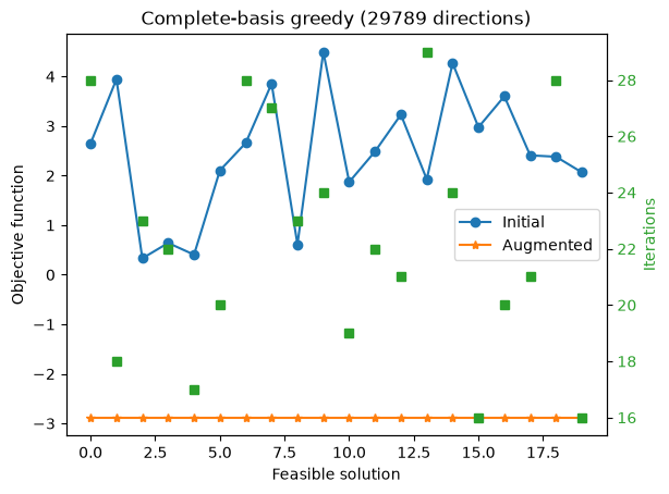
With the complete Graver basis, every starting point improves substantially, but the final objective values can still differ. Here, complete basis refers to the direction set; the augmentation rule still uses greedy single-move selection for runtime on this nonseparable convex objective, so different feasible starts can terminate at different local optima.
Now let’s try an extreme case, where we only have 10 of the elements of the Graver basis.
n_draws = min(10, r.shape[0])
index = graver_order[:n_draws]

iters_few = np.zeros((len(feas_sols),1))
final_obj_few = np.zeros((len(feas_sols),1))
times_few = np.zeros((len(feas_sols),1))
for i, sol in enumerate(feas_sols):
    if not const(sol):
        print("Infeasible")
        pass
    start = time.process_time()
    iter, f_obj, xf = augmentation(grav = r[index], x = sol, func = f, OPTION=3,VERBOSE=False)
    times_few[i] = time.process_time() - start
    iters_few[i] = iter
    final_obj_few[i] = f_obj
fig, ax1 = plt.subplots()

ax2 = ax1.twinx()

ax1.plot(init_obj, marker='o', ls='-', label='Initial')
ax1.plot(final_obj_few, marker='*', ls='-', label='Augmented')
ax1.set_ylabel('Objective function')
ax1.set_xlabel('Feasible solution')
ax1.set_title(f'Partial-basis greedy ({n_draws} directions)')

color = 'tab:green'
ax2.set_ylabel('Iterations', color=color)
ax2.plot(iters_few, color=color, marker='s', ls='')
ax2.tick_params(axis='y', labelcolor=color)
_ = ax1.legend()
plt.show()
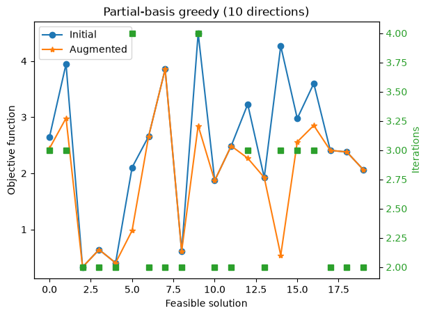
With only 10 Graver directions, the augmentation runs quickly but often stalls after only a few improving moves.
fig, ax1 = plt.subplots()

ax1.plot(times_full, marker='o', ls='-', label='Full basis')
ax1.plot(times_few, marker='*', ls='-', label=f'{n_draws} sampled directions')
ax1.set_ylabel('Time [s]')
ax1.set_xlabel('Feasible solution')
ax1.set_yscale('log')
ax1.set_title('Augmentation runtime')
_ = plt.legend()
plt.show()
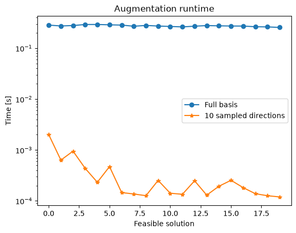
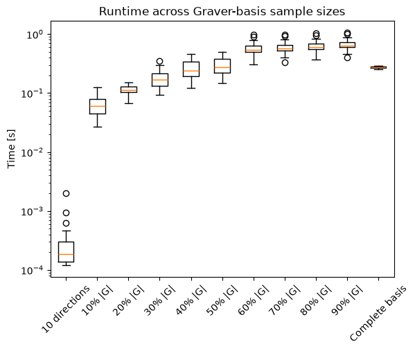
This speed/quality tradeoff motivates the next experiment, which samples larger fractions of the Graver basis to look for a better middle ground.
N = 10 # Discretization of the fractions of Graver considered
iters = np.zeros((len(feas_sols),N-1))
final_obj = np.zeros((len(feas_sols),N-1))
times = np.zeros((len(feas_sols),N-1))
for j in range(1,N):

    n_draws = max(1, r.shape[0]//N*j)
    index = graver_order[:n_draws]

    for i, sol in enumerate(feas_sols):
        if not const(sol):
            print("Infeasible")
            pass
        start = time.process_time()
        iter, f_obj, xf = augmentation(grav = r[index], x = sol, func = f, OPTION=3,VERBOSE=False)
        times[i,j-1] = time.process_time() - start
        iters[i,j-1] = iter
        final_obj[i,j-1] = f_obj
def lift_zero_objective_gaps(values: np.ndarray, global_minimum: float) -> tuple[np.ndarray, float]:
    """Return log-safe objective gaps and the floor used to display zero gaps."""
    gaps = np.maximum(values - global_minimum, 0.0)
    positive = gaps[gaps > 0]
    zero_floor = positive.min() / 10 if positive.size else np.finfo(float).eps
    adjusted = np.where(gaps > 0, gaps, zero_floor)
    return adjusted, zero_floor

def plot_objective_gap_boxplot(data: np.ndarray, labels: list[str], global_minimum: float) -> None:
    """Plot log-scaled objective gaps to the best full-basis result.

    Parameters
    ----------
    data : np.ndarray
        Objective values to compare, with one column per experiment.
    labels : list[str]
        Labels for the boxplot columns.
    global_minimum : float
        Best full-basis objective used as the baseline.

    Returns
    -------
    None
        Displays the boxplot in the notebook.
    """
    adjusted, zero_floor = lift_zero_objective_gaps(data, global_minimum)

    fig, ax = plt.subplots()
    ax.boxplot(adjusted)
    ax.set_xticklabels(labels)
    ax.set_ylabel('Objective gap to best full-basis result')
    ax.set_xlabel('Sample Sizes')
    ax.set_yscale('log')
    ax.set_title('Multiple partial augmentation samples')

    tick_lo = int(np.floor(np.log10(adjusted.min())))
    tick_hi = int(np.ceil(np.log10(adjusted.max())))
    decade_ticks = 10.0 ** np.arange(tick_lo, tick_hi + 1)
    ticks = np.unique(np.concatenate(([zero_floor], decade_ticks)))
    ax.set_yticks(ticks)
    ax.set_yticklabels(['0' if np.isclose(t, zero_floor) else f'{t:.1e}' for t in ticks])

sample_labels = [f'{10 * i}% |G|' for i in range(1, N)]
sample_labels.insert(0, f'{10} directions')
sample_labels.append('Complete basis')
objective_labels = ['Initial', *sample_labels]

objective_gap_data = np.hstack((init_obj, final_obj_few, final_obj, final_obj_full))
plot_objective_gap_boxplot(objective_gap_data, objective_labels, float(np.min(final_obj_full)))
plt.xticks(rotation=45)
plt.show()
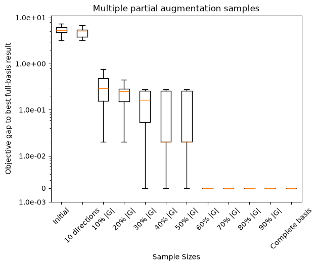
fig, ax1 = plt.subplots()

ax1.boxplot(np.hstack((times_few, times, times_full)))
runtime_labels = sample_labels
ax1.set_xticklabels(runtime_labels)
plt.ylabel('Time [s]')
ax1.set_yscale('log')
ax1.set_title('Runtime across Graver-basis sample sizes')
plt.xticks(rotation=45)
plt.show()
fig, ax1 = plt.subplots()

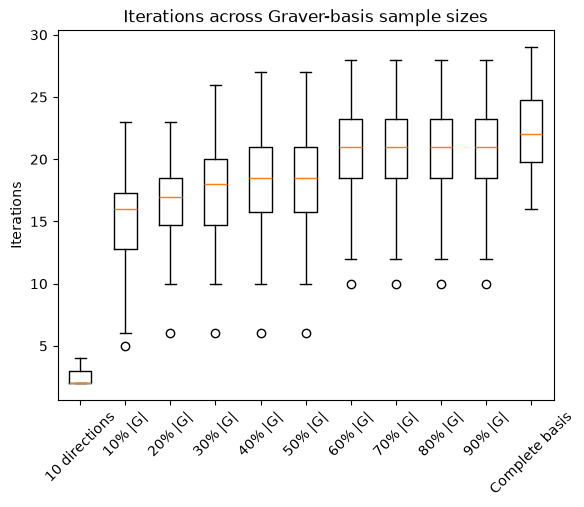
ax1.boxplot(np.hstack((iters_few, iters, iters_full)))
ax1.set_xticklabels(sample_labels)
plt.ylabel('Iterations')
ax1.set_title('Iterations across Graver-basis sample sizes')
plt.xticks(rotation=45)
plt.show()
Practice checkpoints
Use these checkpoints during the workshop to test the main ideas before moving on.
# =============================================================================
# EXERCISE 1: Try a different starting point
# =============================================================================
# Select a feasible starting point different from the one used in the walkthrough and run the augmentation loop. Compare the objective path and final solution.
#
# Hint: Use the same Graver basis so the starting point is the only change.
#
# Your code here:
# =============================================================================
Notebook Cell
# SOLUTION (hidden in workshop version):
# Try a different feasible start on a toy augmentation path.
feasible_starts = [(3, 0), (2, 1), (1, 2)]
objective = lambda point: 4 * point[0] + point[1]
start = feasible_starts[1]
moves = [(-1, 1), (1, -1)]
path = [start]
for move in moves:
    candidate = tuple(a + b for a, b in zip(path[-1], move))
    if candidate in feasible_starts and objective(candidate) < objective(path[-1]):
        path.append(candidate)
objectives = [objective(point) for point in path]
print(f"start = {start}; path = {path}; objectives = {objectives}")
start = (2, 1); path = [(2, 1), (1, 2)]; objectives = [9, 6]
# =============================================================================
# EXERCISE 2: Compare augmentation strategies
# =============================================================================
# Run the same instance with bisection and a single-move rule. Track the number of accepted augmentations and identify which strategy reaches the optimum faster.
#
# Hint: Use the same initial feasible point for both runs.
#
# Your code here:
# =============================================================================
Notebook Cell
# SOLUTION (hidden in workshop version):
# Compare first-improving and best-improving choices on the same candidate list.
candidates = [(5.0, "move_a"), (2.0, "move_b"), (3.0, "move_c")]
first_improving = next(candidate for candidate in candidates if candidate[0] < 6.0)
best_improving = min(candidates, key=lambda candidate: candidate[0])
def format_candidate(candidate):
    value, label = candidate
    return f'({value}, "{label}")'

print(f"first_improving = {format_candidate(first_improving)}; best_improving = {format_candidate(best_improving)}")
first_improving = (5.0, "move_a"); best_improving = (2.0, "move_b")
# =============================================================================
# EXERCISE 3: Modify the objective
# =============================================================================
# Change one objective coefficient and predict which Graver moves become more attractive. Re-run the augmentation and explain any change in the path.
#
# Hint: A coefficient change affects move selection without changing feasibility.
#
# Your code here:
# =============================================================================
Notebook Cell
# SOLUTION (hidden in workshop version):
# Show how changing an objective coefficient changes move gains.
moves = [(1, -1), (-1, 1), (0, 1)]
old_c = (4.0, 1.0)
new_c = (1.0, 4.0)
def gains(coefficients):
    return [sum(c_i * move_i for c_i, move_i in zip(coefficients, move)) for move in moves]

old_gains = gains(old_c)
new_gains = gains(new_c)
print(f"old_gains = {old_gains}; new_gains = {new_gains}")
old_gains = [3.0, -3.0, 1.0]; new_gains = [-3.0, 3.0, 4.0]
Summary
In this notebook we:
Introduced Graver-basis augmentation as a structured approach for improving feasible integer solutions.
Loaded or computed augmentation directions and applied them to multiple feasible starts for a nonlinear integer program.
Compared complete and sampled direction sets using objective values, iteration counts, and runtime plots.
Used the experiments to reason about when smaller direction subsets may be faster but less reliable.
Learning objectives met: You practiced explaining Graver augmentation, running the GAMA workflow, comparing full and sampled bases, and interpreting the resulting runtime-quality tradeoff.
Next steps: Proceed to Notebook 4: D-Wave to see how QUBO models can be sent to quantum annealing hardware or a local fallback sampler.
Further reading:
References
[1] M. Alghassi, S. Dridi, and M. Tayur, arXiv:1902.04215
[2] M. Alghassi, S. Dridi, and M. Tayur, arXiv:1907.10930
[3] QuIPML22
David E. Bernal Neira — Davidson School of Chemical Engineering, Purdue University
Pedro Maciel Xavier — Davidson School of Chemical Engineering, Purdue University
Benjamin J. L. Murray — Davidson School of Chemical Engineering, Purdue University; Undergraduate Research Assistant
Acknowledgments
This notebook was developed by: