
Setup
Google Colab
Click the badge above to open this notebook in Colab. The setup cell installs the local simulated-annealing dependencies.
Local installation
Run the following from the repository root before opening this notebook locally (Python 3.10–3.12):
uv sync --locked --group docs --group qubo
uv run --locked --group docs --group qubo jupyter lab
make verify-dwave-python-local executes the complete local path into .nbverify/ without QPU access. The optional hardware cells require a separately managed Ocean installation and an explicit opt-in; see the quantum-annealing section below.
Learning objectives
By the end of this notebook you will be able to:
Prepare a QUBO/BQM for submission through D-Wave Ocean tools.
Distinguish local simulated annealing from quantum annealing on D-Wave hardware.
Inspect QPU topology, embeddings, and chain-related sampling metadata when a solver is available.
Explain how annealing time, chain strength, and annealing schedules can affect sampling behavior.
Compare a prescribed quantum annealing schedule with an optional QAOA circuit on the same QUBO.
Prerequisites
Mathematical background: QUBO models, graph representations, and the penalty-model ideas from Notebook 2.
Prior notebooks: Notebook 2 (QUBO); Notebook 3 is useful for comparing solver strategies.
Accounts required: A D-Wave Leap account and DWAVE_API_TOKEN for QPU sections; local cells run without an account or token.
Python version: Python 3.10–3.12; local dependencies are locked in the docs and qubo groups.
This notebook introduces D-Wave’s quantum annealing workflow. We formulate the earlier QUBO example with dimod, solve it locally with neal simulated annealing, and optionally submit it to a D-Wave quantum processing unit. We also use NetworkX to represent and visualize graphs.
Problem statement
We define a QUBO as the following optimization problem:
where we optimize over binary variables , on a constrained graph defined by an adjacency matrix . We also include an arbitrary offset .
Example
Suppose we want to solve the following problem via QUBO $$ \min_{\mathbf{x}} 2𝑥_0+4𝑥_1+4𝑥_2+4𝑥_3+4𝑥_4+4𝑥_5+5𝑥_6+4𝑥_7+5𝑥_8+6𝑥_9+5𝑥_{10} \ s.t. \begin{bmatrix} 1 & 0 & 0 & 1 & 1 & 1 & 0 & 1 & 1 & 1 & 1\ 0 & 1 & 0 & 1 & 0 & 1 & 1 & 0 & 1 & 1 & 1\ 0 & 0 & 1 & 0 & 1 & 0 & 1 & 1 & 1 & 1 & 1 \end{bmatrix}\mathbf{x}=
\mathbf{x} \in {0,1 }^{11} $$
Notebook Cell
# If using this on Google Colab, we need to install the packages
try:
  import google.colab
  IN_COLAB = True
except ImportError:
  IN_COLAB = False

if IN_COLAB:
    !pip install -q dimod dwave-neal scipy pandas networkx matplotlib
# Import the Dwave packages dimod and neal
import dimod
import neal
# Import Matplotlib to generate plots
import matplotlib.pyplot as plt
# Import numpy and scipy for certain numerical calculations below
import numpy as np
from collections import Counter
import pandas as pd
import networkx as nxFirst, we rewrite this problem as an unconstrained one by adding quadratic penalties for the linear constraints. Let’s define the problem parameters.
A = np.array([[1, 0, 0, 1, 1, 1, 0, 1, 1, 1, 1],
            [0, 1, 0, 1, 0, 1, 1, 0, 1, 1, 1],
            [0, 0, 1, 0, 1, 0, 1, 1, 1, 1, 1]])
b = np.array([1, 1, 1])
c = np.array([2, 4, 4, 4, 4, 4, 5, 4, 5,6, 5])
In order to define the matrix, we write the problem
as follows:
Exploting the fact that for , we can make the linear terms appear in the diagonal of the matrix.
Penalty parameter rationale
The penalty term must be large enough that any infeasible assignment is worse than the objective improvement it might gain by violating the constraint. For a binary constraint A x = b, the residual A x - b is integer-valued; the smallest nonzero violation has squared penalty at least 1. A conservative sufficient bound is rho = sum(abs(c)) + epsilon, because changing binary variables can improve the linear objective by at most sum(abs(c_i)).
Worked example: if sum(abs(c_i)) = 6 and rho = 5.9, an infeasible assignment with violation 1 can gain 6 objective units while paying only 5.9 penalty units, so it can look 0.1 units better than a feasible assignment. Choosing rho = 6 + epsilon closes that gap for this bounded binary model.
This is a sufficient bound for this model family, not a universal rule. Constraints with non-binary variables, non-integer residuals, or a larger objective range need a problem-specific penalty analysis. See Glover, Kochenberger, and Du (2019), “A Tutorial on Formulating and Using QUBO Models.”
epsilon = 1
rho = np.sum(np.abs(c)) + epsilon
Q = rho*np.matmul(A.T,A)
Q += np.diag(c)
Q -= rho*2*np.diag(np.matmul(b.T,A))
cQ = rho*np.matmul(b.T,b)
print(Q)
print(cQ)
[[ -46    0    0   48   48   48    0   48   48   48   48]
 [   0  -44    0   48    0   48   48    0   48   48   48]
 [   0    0  -44    0   48    0   48   48   48   48   48]
 [  48   48    0  -92   48   96   48   48   96   96   96]
 [  48    0   48   48  -92   48   48   96   96   96   96]
 [  48   48    0   96   48  -92   48   48   96   96   96]
 [   0   48   48   48   48   48  -91   48   96   96   96]
 [  48    0   48   48   96   48   48  -92   96   96   96]
 [  48   48   48   96   96   96   96   96 -139  144  144]
 [  48   48   48   96   96   96   96   96  144 -138  144]
 [  48   48   48   96   96   96   96   96  144  144 -139]]
144
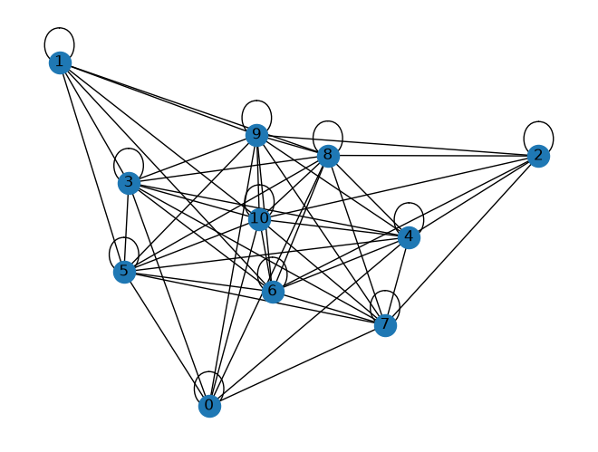
We can visualize the graph that defines this instance using the Q matrix as the adjacency matrix of a graph.
G = nx.from_numpy_array(Q)
# A fixed layout seed makes the drawing repeatable.
nx.draw(G, pos=nx.spring_layout(G, seed=314159), with_labels=True)
Let’s define a QUBO model and then solve it via simulated annealing.
model = dimod.BinaryQuadraticModel.from_qubo(Q, offset=cQ)def plot_enumerate(results, title=None):
plt.figure()
energies = [datum.energy for datum in results.data(
['energy'], sorted_by=None)]
if results.vartype == 'Vartype.BINARY':
samples = [''.join(c for c in str(datum.sample.values()).strip(
', ') if c.isdigit()) for datum in results.data(['sample'], sorted_by=None)]
plt.xlabel('bitstring for solution')
else:
samples = np.arange(len(energies))
plt.xlabel('solution')
plt.bar(samples,energies)
plt.xticks(rotation=90)
plt.ylabel('Energy')
plt.title(str(title))
print("minimum energy:", min(energies))
def plot_energies(results, title=None):
energies = results.data_vectors['energy']
occurrences = results.data_vectors['num_occurrences']
counts = Counter(energies)
total = sum(occurrences)
counts = {}
for index, energy in enumerate(energies):
if energy in counts.keys():
counts[energy] += occurrences[index]
else:
counts[energy] = occurrences[index]
for key in counts:
counts[key] /= total
df = pd.DataFrame.from_dict(counts, orient='index').sort_index()
df.plot(kind='bar', legend=None)
plt.xlabel('Energy')
plt.ylabel('Probabilities')
plt.title(str(title))
plt.show()
print("minimum energy:", min(energies))Let’s now solve this problem using Simulated Annealing
# A fixed seed makes the local sampling repeatable.
simAnnSampler = neal.SimulatedAnnealingSampler()
simAnnSamples = simAnnSampler.sample(model, num_reads=1000, seed=314159)

# This example has only 11 binary variables (2048 states), so we can check
# the sampler against exhaustive enumeration, including the QUBO offset.
exactSamples = dimod.ExactSolver().sample(model)
assert len(exactSamples) == 2 ** len(c)
assert simAnnSamples.record.num_occurrences.sum() == 1000
np.testing.assert_allclose(simAnnSamples.record.energy, model.energies(simAnnSamples))
np.testing.assert_allclose(simAnnSamples.first.energy, exactSamples.first.energy)
best_x = np.array([simAnnSamples.first.sample[i] for i in range(len(c))])
np.testing.assert_array_equal(A @ best_x, b)
np.testing.assert_allclose(c @ best_x, simAnnSamples.first.energy)
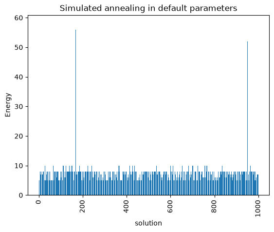
plot_enumerate(simAnnSamples, title='Simulated annealing in default parameters')
plot_energies(simAnnSamples, title='Simulated annealing in default parameters')
minimum energy: 5.0
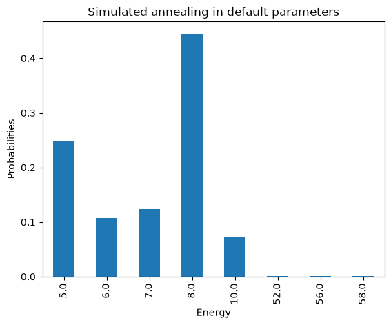
minimum energy: 5.0
Now let’s solve this using Quantum Annealing!
The default execution stays local: it skips account discovery, connectivity checks, and QPU submission, then uses seeded SimulatedAnnealingSampler samples. The saved QPU topology, embedding, and sampling outputs below are historical results from an earlier hardware run. They are retained for the published lesson; a fresh local run produces skip messages and classical sampling plots instead.
To deliberately run the hardware demonstration, use a separately managed Ocean environment and set QUBONOTEBOOKS_DWAVE_ENABLE_QPU=1 before running the notebook. The locked local environment excludes the Ocean cloud client; see local setup. QPU jobs consume access and credits, and an opted-in connection or submission failure raises an error.
Create a D-Wave Leap account at https://DWAVE_API_TOKEN through your process environment, or store it in Colab Secrets under that name. Do not paste a token into a notebook cell. Existing Ocean local configuration remains supported when you opt in without this environment variable. The guarded dwave ping diagnostic uses the same configuration.
# Configure credentials only after explicit QPU opt-in.
import os

enable_qpu = os.environ.get("QUBONOTEBOOKS_DWAVE_ENABLE_QPU", "0") == "1"
api_token = ""
if enable_qpu:
    api_token = os.environ.get("DWAVE_API_TOKEN", "")
    if IN_COLAB:
        from google.colab import userdata
        try:
            api_token = userdata.get("DWAVE_API_TOKEN") or api_token
        except (userdata.SecretNotFoundError, userdata.NotebookAccessError):
            pass  # An opted-in run can still use Ocean's local configuration.
    if api_token:
        os.environ["DWAVE_API_TOKEN"] = api_token
else:
    print("D-Wave QPU disabled; running local simulated annealing only.")
# Verify connectivity only for an explicitly requested hardware run.
import subprocess

if enable_qpu:
    subprocess.run(["dwave", "ping"], check=True)
else:
    print("Skipping `dwave ping`: QPU access is disabled.")
Using endpoint: https://cloud.dwavesys.com/sapi/
Using region: na-west-1
Using solver: Advantage2_system1
Working graph version: 01138bbada
Submitted problem ID: 2456d588-e031-485f-ae03-25e3e639fb12
Wall clock time:
 * Solver definition fetch: 326.372 ms
 * Problem submit and results fetch: 521.775 ms
 * Total: 848.148 ms

QPU timing:
 * post_processing_overhead_time = 1.0 us
 * qpu_access_overhead_time = 734.24 us
 * qpu_access_time = 34690.76 us
 * qpu_anneal_time_per_sample = 20.0 us
 * qpu_delay_time_per_sample = 60.57 us
 * qpu_programming_time = 34586.8 us
 * qpu_readout_time_per_sample = 23.39 us
 * qpu_sampling_time = 103.96 us
 * total_post_processing_time = 1.0 us
from pprint import pprint

if enable_qpu:
    from dwave.system import DWaveSampler, EmbeddingComposite
# Graph corresponding to the selected D-Wave QPU, or a local fallback when unavailable.
qpu = None
qpu_available = False
topology_type = None
X = None


def topology_position_map(graph):
    nodes = sorted(graph.nodes(), key=lambda node: str(node))
    if not nodes:
        return {}
    columns = int(np.ceil(np.sqrt(len(nodes))))
    return {node: (index % columns, -(index // columns)) for index, node in enumerate(nodes)}


def topology_title(topology_type):
    if topology_type == "chimera":
        return "Chimera QPU topology (schematic layout)"
    if topology_type == "pegasus":
        return "Pegasus QPU topology (schematic layout)"
    if topology_type == "zephyr":
        return "Zephyr QPU topology (schematic layout)"
    return "D-Wave QPU topology (schematic layout)"


def draw_topology_graph(graph, *, topology_type=None, node_size=1):
    if graph is None or graph.number_of_nodes() == 0:
        print("No D-Wave QPU topology graph is available to draw.")
        return

    pos = topology_position_map(graph)
    plt.figure(figsize=(7, 5))
    nx.draw_networkx_edges(graph, pos=pos, width=0.05, alpha=0.2)
    nx.draw_networkx_nodes(graph, pos=pos, node_size=node_size, node_color="tab:blue")
    plt.title(topology_title(topology_type))
    plt.axis("off")


if enable_qpu:
    if api_token:
        qpu = DWaveSampler(token=api_token, solver={"qpu": True})
    else:
        qpu = DWaveSampler(solver={"qpu": True})

    topology = qpu.properties["topology"]
    topology_type = topology["type"]
    topology_shape = topology["shape"]
    qpu_edges = qpu.edgelist
    qpu_nodes = qpu.nodelist
    X = qpu.to_networkx_graph()
    qpu_available = True

    print("Solver id:    ", qpu.solver.identity)
    print("Topology:     ", topology_type, "shape=", topology_shape)
    print("Number of qubits=", len(qpu_nodes))
    print("Number of couplers=", len(qpu_edges))

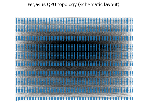
    draw_topology_graph(X, topology_type=topology_type, node_size=1)
else:
    print("Skipping QPU topology discovery: QPU access is disabled.")
Solver id:     Advantage_system4;graph_id=01d07086e1
Topology:      pegasus shape= [16]
Number of qubits= 5627
Number of couplers= 40279
if qpu_available:
    DWavesampler = EmbeddingComposite(qpu)
    DWaveSamples = DWavesampler.sample(
        bqm=model,
        num_reads=1000,
        return_embedding=True,
        # chain_strength=chain_strength,
        # annealing_time=annealing_time,
    )
else:
    DWavesampler = neal.SimulatedAnnealingSampler()
    DWaveSamples = DWavesampler.sample(model, num_reads=1000, seed=314159)
    np.testing.assert_allclose(DWaveSamples.first.energy, exactSamples.first.energy)
print(DWaveSamples.info){'timing': {'qpu_sampling_time': 88880.0, 'qpu_anneal_time_per_sample': 20.0, 'qpu_readout_time_per_sample': 48.3, 'qpu_access_time': 104642.76, 'qpu_access_overhead_time': 724.24, 'qpu_programming_time': 15762.76, 'qpu_delay_time_per_sample': 20.58, 'total_post_processing_time': 1.0, 'post_processing_overhead_time': 1.0}, 'problem_id': '2a51da6a-6066-4e2a-b24c-1eb9d5d7ef64', 'embedding_context': {'embedding': {3: (3835,), 0: (3715, 1924), 1: (3820,), 4: (1939, 3700), 2: (1984,), 5: (1909, 3865), 6: (3760, 1969), 7: (1985, 3850), 8: (3805, 1954), 9: (2000, 1999), 10: (3790, 1894)}, 'chain_break_method': 'majority_vote', 'embedding_parameters': {}, 'chain_strength': 159.83033942960208, 'timing': {'embedding': 0.0007941749645397067, 'unembedding': 0.0005198059370741248}}}
def draw_embedding_graph(graph, embedding, *, topology_type=None, node_size=2):
    if graph is None or not embedding:
        print("No D-Wave QPU embedding graph is available to draw.")
        return

    embedded_nodes = set()
    for chain in embedding.values():
        embedded_nodes.update(chain)

    pos = topology_position_map(graph)
    embedded_nodelist = [node for node in embedded_nodes if node in graph]
    plt.figure(figsize=(7, 5))
    nx.draw_networkx_edges(graph, pos=pos, width=0.05, alpha=0.15)
    nx.draw_networkx_nodes(graph, pos=pos, node_size=node_size, node_color="lightgray")
    nx.draw_networkx_nodes(
        graph,
        pos=pos,
        nodelist=embedded_nodelist,
        node_size=max(node_size * 4, 8),
        node_color="tab:red",
    )
    plt.title(f"{topology_title(topology_type)} with embedding")
    plt.axis("off")


if qpu_available and "embedding_context" in DWaveSamples.info:
    embedding = DWaveSamples.info["embedding_context"]["embedding"]
    draw_embedding_graph(X, embedding, topology_type=topology_type, node_size=2)
else:
    print("No D-Wave QPU embedding is available while using SimulatedAnnealingSampler fallback.")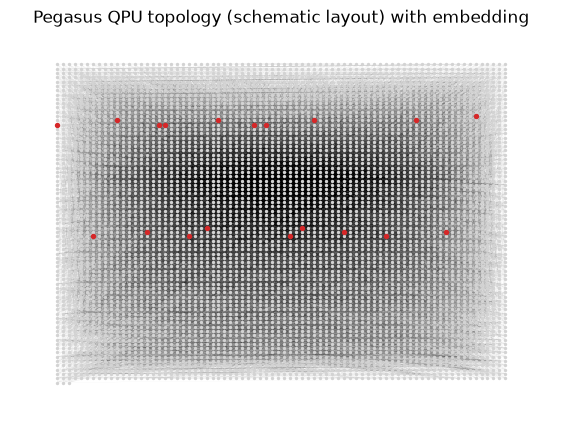
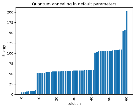
sampling_title = "Quantum annealing in default parameters" if qpu_available else "Simulated annealing (local fallback)"
plot_enumerate(DWaveSamples, title=sampling_title)
plot_energies(DWaveSamples, title=sampling_title)
minimum energy: 5.0
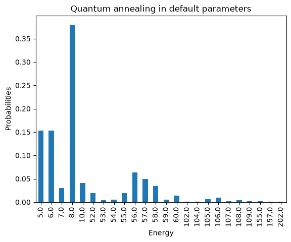
minimum energy: 5.0
Now we can play with the other parameters such as Annealing time, chain strength, and annealing schedule to improve the performance of D-Wave’s Quantum Annealing.
Practice checkpoints
Use these checkpoints during the workshop to test the main ideas before moving on.
# =============================================================================
# EXERCISE 1: Vary the penalty parameter
# =============================================================================
# Change the QUBO penalty parameter and observe how the sampled solutions balance feasibility against objective value. Note whether embedding metadata changes when a QPU is available.
#
# Hint: Use the local simulated annealing fallback if no Leap token is configured.
#
# Your code here:
# =============================================================================
Notebook Cell
# SOLUTION (hidden in workshop version):
# Rebuild a tiny penalty model with two rho values and compare feasibility.
import itertools

def penalty_energy(bits, rho_value):
    x0, x1 = bits
    objective = x0 + 2 * x1
    violation = x0 + x1 - 1
    return objective + rho_value * violation**2

for rho_value in [0.25, 4.0]:
    best = min(
        ((bits, penalty_energy(bits, rho_value)) for bits in itertools.product([0, 1], repeat=2)),
        key=lambda item: item[1],
    )
    feasible = sum(best[0]) == 1
    print(f"rho = {rho_value}; best = {best}; feasible = {str(feasible).lower()}")
rho = 0.25; best = ((0, 0), 0.25); feasible = false
rho = 4.0; best = ((1, 0), 1.0); feasible = true
# =============================================================================
# EXERCISE 2: Sweep the number of reads
# =============================================================================
# Run the sampler with at least three num_reads values and plot the best energy or feasible-solution rate against reads.
#
# Hint: Keep all other sampler parameters fixed.
#
# Your code here:
# =============================================================================
Notebook Cell
# SOLUTION (hidden in workshop version):
# Sweep read counts with a deterministic stand-in for best-energy summaries.
read_counts = [100, 500, 1000]
best_energy_by_reads = {
    reads: min(-1.0, -1.0 - 0.05 * index)
    for index, reads in enumerate(read_counts)
}
formatted_results = ", ".join(f"{reads}: {best_energy_by_reads[reads]}" for reads in read_counts)
print(f"best_energy_by_reads = {{{formatted_results}}}")
best_energy_by_reads = {100: -1.0, 500: -1.05, 1000: -1.1}
# =============================================================================
# EXERCISE 3: Inspect chain behavior
# =============================================================================
# When QPU access is available, compare the returned embedding and chain-related metadata for two chain-strength settings.
#
# Hint: Skip this checkpoint with a written note if only the local fallback sampler is available.
#
# Your code here:
# =============================================================================
Notebook Cell
# SOLUTION (hidden in workshop version):
# Inspect chain behavior only when a QPU sample set is available.
if globals().get("qpu_available") and "embedding_context" in DWaveSamples.info:
    embedding = DWaveSamples.info["embedding_context"]["embedding"]
    chain_lengths = {variable: len(chain) for variable, chain in embedding.items()}
    formatted_lengths = ", ".join(
        f"{variable}: {chain_lengths[variable]}" for variable in sorted(chain_lengths)
    )
    print(f"chain_lengths = {{{formatted_lengths}}}")
else:
    print("QPU embedding metadata is unavailable; use the local fallback result above.")
QPU embedding metadata is unavailable; use the local fallback result above.
Simulating the quantum anneal with CUDA-Q
The local neal runs above use classical simulated annealing. Here we simulate the quantum evolution itself, on a CPU, for the same 11-variable integer program. We will measure the probability of an optimal feasible assignment, inspect the energy spectrum, and sample solutions. Enumerating all assignments provides our correctness reference; this is a teaching example, not a speed comparison with neal or a QPU.
CUDA-Q is optional. From the repository root, make verify-cudaq-python installs the optional group and runs both this annealing section and the QAOA comparison that follows. Without it, the notebook prints Skipping CUDA-Q quantum methods: install the optional cudaq group. and continues. The availability message, numerical outputs, and figure below record one CUDA-Q-enabled CPU run. The missing-package test and D-Wave local CI lane verify the skip path. See local setup for platform and installation details.
From the integer program to the problem Hamiltonian
The model already built above has energy
dimod uses spins when converting a BQM to Ising coefficients. On a computational basis state, Pauli has eigenvalue . Therefore the Hamiltonian for minimization is
The minus sign applies to the linear spin coefficients; the pair terms keep their sign. Its computational-basis energies must equal the original penalized objective, including the offset .
Choose in the model’s arbitrary cost units and use the dimensionless schedule
Here and are dimensionless: physical time would be . They are not D-Wave annealing times in microseconds. The ground state of is with energy , so Hadamard gates prepare the correct initial state. Positive rescaling of preserves its minimizers.
CUDA-Q statevector indices use qubit 0 as the least significant bit; sampled strings list qubit 0 first. We account for both conventions explicitly and check every basis-state energy.
# Optional CUDA-Q import: a broken installation must not become a clean skip.
import os
import warnings

CUDAQ_SKIP_MESSAGE = "Skipping CUDA-Q quantum methods: install the optional cudaq group."
try:
    # CUDA-Q 0.16 emits this notice unconditionally; migration guidance is pending.
    # Filter only this exact import notice, preserving all other warnings.
    with warnings.catch_warnings():
        warnings.filterwarnings(
            "ignore",
            message=(
                r"^The CUDA-Q `sample` and `observe` algorithmic primitives will change in "
                r"a future release\. Existing code may require updates\. See "
                r"https://nvidia\.github\.io/cuda-quantum/latest/using/migration/"
                r"upcoming_changes\.html for details\.$"
            ),
            category=FutureWarning,
        )
        import cudaq
except ModuleNotFoundError as exc:
    if exc.name != "cudaq" or os.environ.get("QUBONOTEBOOKS_CUDAQ_REQUIRE", "0") == "1":
        raise
    HAS_CUDAQ = False
    print(CUDAQ_SKIP_MESSAGE)
else:
    HAS_CUDAQ = True
    cudaq.set_target("qpp-cpu")
    cudaq.set_random_seed(314159)
    print("CUDA-Q enabled: qpp-cpu, ideal noiseless quantum simulation.")
CUDA-Q enabled: qpp-cpu, ideal noiseless quantum simulation.
def ising_cost_data(bqm, energy_scale):
    """Convert contiguous binary variables to Pauli-Z coefficients.

    Parameters
    ----------
    bqm : dimod.BinaryQuadraticModel
        Penalized objective in arbitrary cost units; variables are 0, ..., n-1.
    energy_scale : float
        Positive reference energy in the same cost units.

    Returns
    -------
    fields, left, right, couplings, offset : tuple
        Dimensionless Z fields, paired qubit indices, ZZ couplings, and offset.
        The sign change follows x=(1-Z)/2 and dimod's spin=2*x-1 convention.
    """
    if energy_scale <= 0:
        raise ValueError("The reference energy must be positive.")
    spin_fields, spin_pairs, offset = bqm.to_ising()
    pairs = sorted(spin_pairs)
    return (
        [-float(spin_fields[i]) / energy_scale for i in range(len(bqm))],
        [int(i) for i, j in pairs],
        [int(j) for i, j in pairs],
        [float(spin_pairs[pair]) / energy_scale for pair in pairs],
        float(offset) / energy_scale,
    )


if HAS_CUDAQ:
    n_qubits = len(model)
    energy_scale = float(rho)  # Reference energy, in the original cost units.
    fields, pair_left, pair_right, couplings, ising_offset = ising_cost_data(model, energy_scale)
    basis_indices = np.arange(2 ** n_qubits)
    basis_bits = (basis_indices[:, None] >> np.arange(n_qubits)) & 1
    qubo_energies = model.energies((basis_bits, list(range(n_qubits))))
    direct_energies = basis_bits @ c + rho * np.sum((basis_bits @ A.T - b) ** 2, axis=1)
    np.testing.assert_allclose(qubo_energies, direct_energies)
    ground_energy = qubo_energies.min()
    ground_mask = np.isclose(qubo_energies, ground_energy)
    feasible_mask = np.all(basis_bits @ A.T == b, axis=1)
    assert np.all(feasible_mask[ground_mask])

    problem_hamiltonian = ising_offset * cudaq.spin.i(0)
    mixer_hamiltonian = -cudaq.spin.x(0)
    for i in range(n_qubits):
        problem_hamiltonian += fields[i] * cudaq.spin.z(i)
        if i > 0:
            mixer_hamiltonian -= cudaq.spin.x(i)
    for i, j, coefficient in zip(pair_left, pair_right, couplings):
        problem_hamiltonian += coefficient * cudaq.spin.z(i) * cudaq.spin.z(j)

    # Endpoint check 1: every final Hamiltonian energy is the QUBO cost / E_ref.
    np.testing.assert_allclose(
        np.diag(problem_hamiltonian.to_matrix()).real,
        qubo_energies / energy_scale,
        atol=1e-10,
    )
    print(f"Exact optimum: {ground_energy:g}; feasible minimizers: {ground_mask.sum()}")
    print("Optimal assignments (x0, ..., x10):")
    print(basis_bits[ground_mask])
Exact optimum: 5; feasible minimizers: 2
Optimal assignments (x0, ..., x10):
[[0 0 0 0 0 0 0 0 1 0 0]
 [0 0 0 0 0 0 0 0 0 0 1]]
Follow the annealing schedule with a quantum circuit
For a midpoint and step , use the symmetric product formula
Since , each mixer half-step uses . Problem terms use and a CNOT––CNOT pair. All problem terms commute. The constant offset contributes only a global phase and can be omitted during evolution, while remaining in energy comparisons.
The step size below is at most 0.1 in dimensionless time. During development, this circuit was compared with a direct dense SciPy Schrödinger-equation solution at : the ground-space probability differed by about , falling to when the step size was halved. This is a discretized, finite-time anneal, not an assumption of perfect adiabatic evolution.
if HAS_CUDAQ:
    @cudaq.kernel
    def quantum_anneal(n: int, z_fields: list[float], left: list[int], right: list[int],
                      zz_couplings: list[float], total_time: float, steps: int):
        """Evolve dimensionless H(s) with midpoint symmetric Trotter steps."""
        qubits = cudaq.qvector(n)
        h(qubits)
        dt = total_time / steps
        for k in range(steps):
            s = (k + 0.5) / steps
            for i in range(n):
                rx(-dt * (1.0 - s), qubits[i])
            for i in range(n):
                rz(2.0 * dt * s * z_fields[i], qubits[i])
            for j in range(len(zz_couplings)):
                x.ctrl(qubits[left[j]], qubits[right[j]])
                rz(2.0 * dt * s * zz_couplings[j], qubits[right[j]])
                x.ctrl(qubits[left[j]], qubits[right[j]])
            for i in range(n):
                rx(-dt * (1.0 - s), qubits[i])

    @cudaq.kernel
    def measure_annealed_state(state: cudaq.State):
        """Sample a previously evolved state without repeating the anneal."""
        qubits = cudaq.qvector(state)
        mz(qubits)

    anneal_args = (n_qubits, fields, pair_left, pair_right, couplings)
    # Endpoint check 2: the prepared state is the mixer's ground state.
    initial_energy = cudaq.observe(quantum_anneal, mixer_hamiltonian, *anneal_args, 0.0, 1).expectation()
    np.testing.assert_allclose(initial_energy, -n_qubits, atol=1e-10)

    anneal_runs = []
    for total_time in [0.0, 2.0, 10.0, 50.0, 200.0]:
        steps = max(1, int(np.ceil(total_time / 0.1)))
        final_state = cudaq.get_state(quantum_anneal, *anneal_args, total_time, steps)
        probabilities = np.abs(np.asarray(final_state)) ** 2
        np.testing.assert_allclose(probabilities.sum(), 1.0, atol=1e-8)
        result = {
            "T (dimensionless)": total_time,
            "steps": steps,
            "P(optimal)": float(probabilities[ground_mask].sum()),
            "P(feasible)": float(probabilities[feasible_mask].sum()),
            "mean penalized cost": float(probabilities @ qubo_energies),
        }
        anneal_runs.append((final_state, result))
        if total_time == 0.0:
            np.testing.assert_allclose(result["P(optimal)"], ground_mask.sum() / 2 ** n_qubits)
    # Keep each state paired with its own statistics, even if the time list is reordered.
    longest_anneal_state, longest_anneal_result = max(
        anneal_runs, key=lambda run: run[1]["T (dimensionless)"]
    )
    anneal_results = [result for state, result in anneal_runs]
    assert longest_anneal_result["P(optimal)"] > ground_mask.sum() / 2 ** n_qubits
    print(pd.DataFrame(anneal_results).to_string(index=False, float_format=lambda value: f"{value:.6f}"))
 T (dimensionless)  steps  P(optimal)  P(feasible)  mean penalized cost
          0.000000      1    0.000977     0.004395          1319.500000
          2.000000     20    0.038713     0.176971           215.081707
         10.000000    100    0.120527     0.525642            35.076591
         50.000000    500    0.240729     0.990139             7.684564
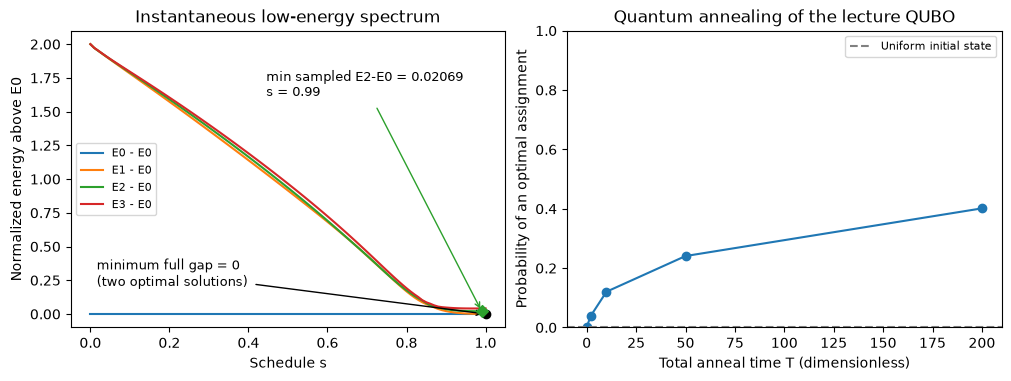
        200.000000   2000    0.401332     0.999282             6.588367
Spectrum, degeneracy, and optimization success
This integer program has two optimal assignments: selecting variable alone or alone gives feasible cost 5. Success therefore means overlap with the entire optimal ground space,
not overlap with one arbitrarily selected eigenvector.
The spectrum below shows the four lowest energies relative to the instantaneous ground energy. Its full gap reaches zero at because those two optima are degenerate. The endpoint gap above the optimal subspace is instead . We also report and mark the minimum sampled value of along the schedule; it is slightly smaller than its endpoint value. This spectral diagnostic does not by itself provide an adiabatic runtime bound. A zero splitting between two successful answers must not be interpreted as failure to reach an optimum, or used blindly in a nondegenerate adiabatic-time estimate. Interior spectral points are sampled numerically; they are not a proof that all interior avoided crossings have been located.
Longer anneals increase success for the settings shown, but finite-time quantum interference need not make every time sweep monotone. This idealized, noiseless, fully connected evolution omits temperature, control errors, and minor embedding. Hardware embedding changes the Hamiltonian and its gaps; the spectrum and schedule help explain why chain strength and annealing time matter in the QPU section above.
if HAS_CUDAQ:
    from scipy.sparse import coo_matrix, diags
    from scipy.sparse.linalg import eigsh

    rows = np.repeat(basis_indices, n_qubits)
    columns = (basis_indices[:, None] ^ (1 << np.arange(n_qubits))).ravel()
    mixer_matrix = coo_matrix(
        (-np.ones(len(rows)), (rows, columns)),
        shape=(len(basis_indices), len(basis_indices)),
    ).tocsr()
    problem_matrix = diags(qubo_energies / energy_scale)
    schedule_points = np.linspace(0.0, 1.0, 101)
    low_spectrum = []
    # A reproducible generic vector explores symmetry sectors that a uniform
    # starting vector could miss. Endpoint degeneracies are known exactly.
    spectral_start = np.random.default_rng(314159).normal(size=len(basis_indices))
    spectral_start /= np.linalg.norm(spectral_start)
    for schedule in schedule_points:
        if schedule == 0.0:
            eigenvalues = np.array([-n_qubits, -n_qubits + 2, -n_qubits + 2, -n_qubits + 2], dtype=float)
        elif schedule == 1.0:
            eigenvalues = np.sort(qubo_energies / energy_scale)[:4]
        else:
            instantaneous = (1 - schedule) * mixer_matrix + schedule * problem_matrix
            eigenvalues, eigenvectors = eigsh(instantaneous, k=4, which="SA", tol=1e-9, v0=spectral_start)
            residual = instantaneous @ eigenvectors - eigenvectors * eigenvalues
            assert np.max(np.linalg.norm(residual, axis=0)) < 1e-6
            eigenvalues = np.sort(eigenvalues)
        low_spectrum.append(eigenvalues)
    low_spectrum = np.array(low_spectrum)
    relative_spectrum = low_spectrum - low_spectrum[:, :1]
    minimum_gap_index = int(np.argmin(relative_spectrum[:, 1]))
    endpoint_ground_rank = int(ground_mask.sum())
    # Energies are normalized by E_ref; schedule positions are dimensionless.
    optimal_subspace_gaps = relative_spectrum[:, endpoint_ground_rank]
    minimum_optimal_gap_index = int(np.argmin(optimal_subspace_gaps))
    minimum_optimal_gap = float(optimal_subspace_gaps[minimum_optimal_gap_index])
    minimum_optimal_gap_schedule = float(schedule_points[minimum_optimal_gap_index])
    endpoint_gap = (np.min(qubo_energies[~ground_mask]) - ground_energy) / energy_scale
    np.testing.assert_allclose(relative_spectrum[-1, :endpoint_ground_rank], 0.0, atol=1e-10)
    print(f"Minimum full gap E1-E0: {relative_spectrum[minimum_gap_index, 1]:.6f} at s={schedule_points[minimum_gap_index]:.2f}")
    print(f"Endpoint gap above the optimal subspace: {endpoint_gap:.6f} (normalized energy)")
    print(f"Minimum sampled E2-E0: {minimum_optimal_gap:.6f} at s={minimum_optimal_gap_schedule:.2f} (normalized energy)")

    fig, axes = plt.subplots(1, 2, figsize=(10, 3.7), constrained_layout=True)
    for level in range(4):
        axes[0].plot(schedule_points, relative_spectrum[:, level], label=f"E{level} - E0")
    axes[0].scatter([1.0], [0.0], color="black", zorder=5)
    axes[0].annotate("minimum full gap = 0\n(two optimal solutions)", xy=(1.0, 0.0),
                     xytext=(0.06, 0.14), textcoords="axes fraction",
                     bbox={"facecolor": "white", "edgecolor": "none", "alpha": 0.95},
                     arrowprops={"arrowstyle": "->"}, fontsize=9)
    axes[0].scatter([minimum_optimal_gap_schedule], [minimum_optimal_gap],
                    color="tab:green", marker="D", zorder=6)
    axes[0].annotate(f"min sampled E2-E0 = {minimum_optimal_gap:.5f}\ns = {minimum_optimal_gap_schedule:.2f}",
                     xy=(minimum_optimal_gap_schedule, minimum_optimal_gap),
                     xytext=(0.45, 0.78), textcoords="axes fraction",
                     bbox={"facecolor": "white", "edgecolor": "none", "alpha": 0.95},
                     arrowprops={"arrowstyle": "->", "color": "tab:green"}, fontsize=9)
    axes[0].set(xlabel="Schedule s", ylabel="Normalized energy above E0", title="Instantaneous low-energy spectrum")
    axes[0].legend(fontsize=8)
    axes[1].plot([row["T (dimensionless)"] for row in anneal_results],
                 [row["P(optimal)"] for row in anneal_results], marker="o")
    axes[1].axhline(ground_mask.sum() / 2 ** n_qubits, color="gray", linestyle="--", label="Uniform initial state")
    axes[1].set(xlabel="Total anneal time T (dimensionless)", ylabel="Probability of an optimal assignment",
                ylim=(0, 1), title="Quantum annealing of the lecture QUBO")
    axes[1].legend(fontsize=8)
    plt.show()
Minimum full gap E1-E0: 0.000000 at s=1.00
Endpoint gap above the optimal subspace: 0.020833 (normalized energy)
Minimum sampled E2-E0: 0.020693 at s=0.99 (normalized energy)
Decode the quantum samples into integer-program solutions
We now sample the explicitly selected longest-anneal state, retained together with its exact probabilities, and map each bit back to the corresponding decision variable. The check uses the original constraints and objective , as well as the QUBO ground energy. The exact statevector probabilities describe the simulator; the counts are a finite-shot estimate. Neither is a claim of quantum advantage.
if HAS_CUDAQ:
    shots = 4096
    anneal_counts = dict(cudaq.sample(measure_annealed_state, longest_anneal_state, shots_count=shots).items())
    assert sum(anneal_counts.values()) == shots
    # CUDA-Q strings put qubit 0 first, unlike integer statevector indexing.
    decoded_samples = {bits: np.array([int(bit) for bit in bits]) for bits in anneal_counts}
    sampled_costs = {
        bits: float(c @ assignment + rho * np.sum((A @ assignment - b) ** 2))
        for bits, assignment in decoded_samples.items()
    }
    best_bits = min(sampled_costs, key=sampled_costs.get)
    best_assignment = decoded_samples[best_bits]
    np.testing.assert_array_equal(A @ best_assignment, b)
    np.testing.assert_allclose(c @ best_assignment, ground_energy)
    optimal_reads = sum(count for bits, count in anneal_counts.items() if np.isclose(sampled_costs[bits], ground_energy))
    success_probability = longest_anneal_result["P(optimal)"]
    sampling_tolerance = 6 * np.sqrt(success_probability * (1 - success_probability) / shots) + 2 / shots
    assert abs(optimal_reads / shots - success_probability) < sampling_tolerance
    print(f"Sampled anneal time T: {longest_anneal_result['T (dimensionless)']:g} (dimensionless)")
    print(f"Best sampled assignment (x0 first): {best_bits}")
    print(f"Original objective: {c @ best_assignment:g}; Ax = {A @ best_assignment}")
    print(f"Optimal reads: {optimal_reads}/{shots}; exact state probability: {success_probability:.6f}")
    print("CUDA-Q quantum annealing checks passed.")
Sampled anneal time T: 200 (dimensionless)
Best sampled assignment (x0 first): 00000000001
Original objective: 5; Ax = [1 1 1]
Optimal reads: 1660/4096; exact state probability: 0.401332
CUDA-Q quantum annealing checks passed.
The circuit implements the product-formula construction described in NVIDIA’s Hamiltonian simulation documentation, with signs derived here for minimization and the original lecture model. CUDA-Q’s execution and bit-ordering conventions explain the distinction between statevector indices and sampled strings.
Optional comparison: QAOA with CUDA-Q
The annealing demonstration followed a prescribed schedule. QAOA (the Quantum Approximate Optimization Algorithm) instead alternates cost and mixer layers, adjusts their angles with a classical optimizer, and measures candidate assignments. We reuse the same 11-variable QUBO, Pauli coefficients, and exact baseline from the annealing section so the change of method is easy to follow. Both are ideal, noiseless CPU simulations; neither establishes a speedup over classical solvers.
This optional comparison uses the CUDA-Q setup above. Without the optional package, both quantum sections skip after one notice. The published results show an enabled CPU run; make verify-cudaq-python reproduces and checks both methods. Students can continue directly to benchmarking, then revisit circuit methods in the Julia QAOA notebook.
The alternating circuit follows Farhi, Goldstone, and Gutmann (2014), A Quantum Approximate Optimization Algorithm.
Reuse the annealing problem Hamiltonian
The earlier mapping already checked all Hamiltonian energies against this QUBO and the original penalty formula. Reuse its dimensionless problem_hamiltonian, which represents with . For QAOA, remove only the identity offset to obtain the cost operator :
The identity contributes only a global phase to the circuit. Restore its offset and the energy scale when reporting QUBO costs, including constraint penalties. The raw Ising expectation alone is not the original objective.
if HAS_CUDAQ:
    assert 1 <= n_qubits <= 12
    # Reset seeds so prior annealing samples do not change this comparison.
    cudaq.set_random_seed(314159)
    np.random.seed(314159)
    cost_hamiltonian = problem_hamiltonian - ising_offset * cudaq.spin.i(0)
    print(f"Reusing the {n_qubits}-variable QUBO and exact optimum {ground_energy:g}.")
Reusing the 11-variable QUBO and exact optimum 5.
Alternating cost and mixer layers
Start from using Hadamard gates. Each of the layers applies followed by . Our parameter order is [gamma[0], ..., gamma[p-1], beta[0], ..., beta[p-1]], matching the indices used below. The identity offset contributes only a global phase, so no gate is needed for it.
Since , each field needs rz(2*gamma*field). A CNOT–RZ–CNOT sequence implements each pair term. The mixer uses rx(2*beta). We write these gates directly with @cudaq.kernel; no QAOA solver package is needed. Increasing adds parameters and gates, and need not improve the result of a bounded local optimization.
if HAS_CUDAQ:
    @cudaq.kernel
    def qaoa(n: int, p: int, z_fields: list[float], left: list[int], right: list[int],
             zz_couplings: list[float], parameters: list[float]):
        """Prepare p cost/mixer layers with dimensionless gamma-then-beta angles."""
        qubits = cudaq.qvector(n)
        h(qubits)
        for layer in range(p):
            gamma = parameters[layer]
            beta = parameters[p + layer]
            for i in range(n):
                rz(2.0 * gamma * z_fields[i], qubits[i])
            for j in range(len(zz_couplings)):
                x.ctrl(qubits[left[j]], qubits[right[j]])
                rz(2.0 * gamma * zz_couplings[j], qubits[right[j]])
                x.ctrl(qubits[left[j]], qubits[right[j]])
            for i in range(n):
                rx(2.0 * beta, qubits[i])

    p = 2
    qaoa_args = (n_qubits, p, fields, pair_left, pair_right, couplings)
The classical outer loop
SciPy’s COBYLA optimizer adjusts the angles to minimize cudaq.observe(...).expectation(). On this simulator observe uses the exact state expectation by default; this optimization has no measurement shots. We use three seeded starting points and a fixed evaluation budget because the objective has local minima. A budget stop is reported, and the lowest observed energy is retained.
The expectation is an average over all assignments, not the energy of a returned solution. We compare it with the uniform initial state’s QUBO expectation and verify it independently from the final state probabilities. Only the subsequent sample call uses finite shots. See CUDA-Q’s execution primitives for these semantics.
if HAS_CUDAQ:
    from scipy.optimize import minimize

    def qaoa_expectation(parameters):
        """Evaluate raw dimensionless Ising expectation and retain the best angles."""
        value = float(cudaq.observe(
            qaoa, cost_hamiltonian, *qaoa_args, parameters.tolist()
        ).expectation())
        if value < best_evaluation["energy"]:
            best_evaluation.update(energy=value, parameters=parameters.copy())
        return value

    best_evaluation = {"energy": float("inf"), "parameters": None}
    optimizer_runs = []
    for restart in range(3):
        initial_parameters = np.random.uniform(-0.5, 0.5, 2 * p)
        result = minimize(
            qaoa_expectation, initial_parameters, method="COBYLA",
            options={"maxiter": 150, "rhobeg": 0.25, "tol": 1e-4},
        )
        optimizer_runs.append({"start": restart + 1, "evaluations": result.nfev,
                               "converged": result.success, "message": result.message})
    optimal_parameters = best_evaluation["parameters"].tolist()
    raw_expectation = best_evaluation["energy"]
    mean_qubo_cost = energy_scale * (raw_expectation + ising_offset)
    final_state = cudaq.get_state(qaoa, *qaoa_args, optimal_parameters)
    probabilities = np.abs(np.asarray(final_state)) ** 2
    np.testing.assert_allclose(probabilities.sum(), 1, atol=1e-9)
    np.testing.assert_allclose(mean_qubo_cost, probabilities @ qubo_energies, atol=1e-8)
    assert ground_energy - 1e-8 <= mean_qubo_cost < qubo_energies.mean()
    success_probability = float(probabilities[ground_mask].sum())
    feasibility_probability = float(probabilities[feasible_mask].sum())
    print(pd.DataFrame(optimizer_runs).to_string(index=False))
    print(f"p={p}; parameters (gamma then beta): {np.round(optimal_parameters, 6)}")
    print(f"Raw Ising expectation (dimensionless, no offset): {raw_expectation:.6f}")
    print(f"Mean QUBO cost: {mean_qubo_cost:.6f}; uniform baseline: {qubo_energies.mean():.6f}")
    print(f"Exact state P(optimal): {success_probability:.6f}; P(feasible): {feasibility_probability:.6f}")
start evaluations converged message
1 150 False Return from COBYLA because the objective function has been evaluated MAXFUN times.
2 150 False Return from COBYLA because the objective function has been evaluated MAXFUN times.
3 150 False Return from COBYLA because the objective function has been evaluated MAXFUN times.
p=2; parameters (gamma then beta): [ 0.051586 0.141741 -0.509189 -0.269327]
Raw Ising expectation (dimensionless, no offset): -25.723833
Mean QUBO cost: 84.756034; uniform baseline: 1319.500000
Exact state P(optimal): 0.042601; P(feasible): 0.166546
Sample, decode, and compare with enumeration
cudaq.sample measures the final state in the computational basis (implicitly, because the ansatz has no measurement gates). Its bitstrings list qubit 0 first: the string 100...0 means . That differs from the integer ordering of the matrix/statevector above; we construct the index explicitly to keep the exact probabilities paired with the right sample.
We report the lowest-QUBO-cost observed sample separately from the most frequent sample; frequency is not an optimization objective. count / shots estimates a sample’s probability, while probabilities[index] is its exact simulator probability. P(optimal) sums the probabilities of all degenerate optima. Feasibility means ; subtracting from the QUBO cost recovers the original unpenalized objective.
For this small seeded demonstration we assert that the sampled best reaches the exact optimum and is feasible, without pinning a histogram or selecting one of the degenerate optimal bitstrings. QAOA and finite-shot sampling do not guarantee that outcome on other instances or budgets.
if HAS_CUDAQ:
    shots = 8192
    counts = cudaq.sample(qaoa, *qaoa_args, optimal_parameters, shots_count=shots)
    assert sum(counts.values()) == shots
    sample_rows = []
    for bitstring, count in counts.items():
        bits = np.array([int(bit) for bit in bitstring])
        index = sum(int(bit) << i for i, bit in enumerate(bits))
        qubo_cost = float(model.energy(dict(enumerate(bits))))
        residual = A @ bits - b
        sample_rows.append({
            "bits (x0 first)": bitstring,
            "raw Ising": qubo_cost / energy_scale - ising_offset,
            "QUBO cost": qubo_cost,
            "original cost": float(c @ bits),
            "feasible": bool(np.all(residual == 0)),
            "count": count,
            "sample frequency": count / shots,
            "exact probability": float(probabilities[index]),
        })
    best_sample = min(sample_rows, key=lambda row: (row["QUBO cost"], row["bits (x0 first)"]))
    most_frequent = max(sample_rows, key=lambda row: row["count"])
    np.testing.assert_allclose(best_sample["QUBO cost"], ground_energy, rtol=0, atol=1e-9)
    assert best_sample["feasible"]
    print(f"Final measurement shots: {shots}")
    print(pd.DataFrame([best_sample, most_frequent], index=["lowest cost", "most frequent"]).to_string(
        float_format=lambda value: f"{value:.6f}"
    ))
    print("CUDA-Q QAOA checks passed.")
Final measurement shots: 8192
bits (x0 first) raw Ising QUBO cost original cost feasible count sample frequency exact probability
lowest cost 00000000001 -27.385417 5.000000 5.000000 True 191 0.023315 0.021300
most frequent 00000000000 -24.489583 144.000000 0.000000 False 736 0.089844 0.082723
CUDA-Q QAOA checks passed.
Summary
In this notebook we:
Reused a QUBO/BQM model and sampled it with local simulated annealing and, when credentials are available, D-Wave quantum annealing.
Checked D-Wave configuration and guarded QPU access so local runs can fall back gracefully.
Inspected solver topology, embeddings, returned sample metadata, and energy distributions.
Simulated the same QUBO with an optional CUDA-Q quantum anneal, checked its Ising convention, and measured optimal-solution probability and spectral gaps.
Compared the annealing schedule with optional QAOA, reusing the Hamiltonian and exact baseline while a classical optimizer chooses circuit angles.
Identified annealing controls such as reads, chain strength, annealing time, and schedules for follow-up experiments.
Learning objectives met: You practiced preparing BQMs for Ocean samplers, distinguishing local and QPU execution, inspecting embeddings, and connecting annealing parameters to solver behavior.
Next steps: Proceed to Notebook 5: Benchmarking to compare solver performance with time-to-solution and performance-ratio metrics.
Further reading:
David E. Bernal Neira — Davidson School of Chemical Engineering, Purdue University
Pedro Maciel Xavier — Davidson School of Chemical Engineering, Purdue University
Benjamin J. L. Murray — Davidson School of Chemical Engineering, Purdue University; Undergraduate Research Assistant
Acknowledgments
This notebook was developed by: