
Setup
Google Colab
Click the badge above to open this notebook in Colab. The notebook installs or activates dependencies in the setup cells below.
Local installation
Run the following from the repository root before opening this notebook locally:
julia --project=notebooks_jl -e 'using Pkg; Pkg.instantiate()'See local-setup.md for installing Julia itself and the full local workflow.
GLPK (required for ILP sections):
macOS:
brew install glpkUbuntu/Debian:
sudo apt-get install glpk-utilsWindows: download from http://
winglpk .sourceforge .net/
Colab Instructions
If not in a Colab notebook, continue to the next section.
Work on a copy of this notebook: File > Save a copy in Drive.
Make sure the runtime is set to Julia. If Colab opens a Python runtime, use Runtime > Change runtime type and select Julia.
Execute the following setup cell to clone the repository when needed, activate the shared notebook project, and install dependencies. The first Colab run can take several minutes.
Notebook Cell
function load_qubonotebooks_bootstrap()
    candidates = (
        joinpath(pwd(), "scripts", "notebook_bootstrap.jl"),
        joinpath(pwd(), "..", "scripts", "notebook_bootstrap.jl"),
        joinpath(pwd(), "QUBONotebooks", "scripts", "notebook_bootstrap.jl"),
        joinpath("/content", "QUBONotebooks", "scripts", "notebook_bootstrap.jl"),
    )

    for candidate in candidates
        if isfile(candidate)
            include(candidate)
            return nothing
        end
    end

    in_colab = haskey(ENV, "COLAB_RELEASE_TAG") || haskey(ENV, "COLAB_JUPYTER_IP") || isdir(joinpath("/content", "sample_data"))
    if in_colab
        repo_dir = get(ENV, "QUBONOTEBOOKS_REPO_DIR", joinpath(pwd(), "QUBONotebooks"))
        if !isdir(repo_dir)
            println("[bootstrap] Cloning JuliaQUBO/QUBONotebooks into $repo_dir")
            run(`git clone --quiet --depth 1 https://github.com/JuliaQUBO/QUBONotebooks.git $repo_dir`)
        end
        include(joinpath(repo_dir, "scripts", "notebook_bootstrap.jl"))
        return nothing
    end

    error("Could not locate scripts/notebook_bootstrap.jl from $(pwd()).")
end

load_qubonotebooks_bootstrap()

BOOTSTRAP = Base.invokelatest(QUBONotebooksBootstrap.bootstrap_notebook, "2-QUBO")

QUBONOTEBOOKS_REPO_DIR = BOOTSTRAP.repo_dir
JULIA_NOTEBOOKS_DIR = BOOTSTRAP.notebooks_dir
JULIA_PROJECT_DIR = BOOTSTRAP.project_dir
IN_COLAB = BOOTSTRAP.in_colab;
Activate Environment
Notebook Cell
import Pkg

python_warning_filter = "ignore:invalid escape sequence:SyntaxWarning"
python_warning_filters = String.(filter(!isempty, split(get(ENV, "PYTHONWARNINGS", ""), ",")))
if python_warning_filter ∉ python_warning_filters
    push!(python_warning_filters, python_warning_filter)
    ENV["PYTHONWARNINGS"] = join(python_warning_filters, ",")
end

if @isdefined(JULIA_PROJECT_DIR)
    Pkg.activate(JULIA_PROJECT_DIR; io = devnull)
else
    Pkg.activate(@__DIR__; io = devnull)
end
Pkg.instantiate(; io = devnull, allow_autoprecomp = false)
Learning objectives
By the end of this notebook you will be able to:
Describe QUBO and Ising model forms and the role of linear, quadratic, and offset terms.
Convert constrained binary optimization problems into QUBO models using penalty terms.
Build and solve QUBO/Ising models with JuliaQUBO tooling and simulated annealing.
Validate sampled solutions and connect QUBO penalties to graph-coloring feasibility.
Prerequisites
Mathematical background: Binary variables, matrix notation, quadratic objectives, and basic graph terminology.
Prior notebooks: Notebook 1 (MathProg) or equivalent experience with binary integer programming.
Accounts required: None; all examples use local or Colab Julia packages.
Julia version: Julia 1.10+ with the notebook project and JuliaQUBO packages instantiated.
# QUBONOTEBOOKS_COLAB_IMPORT_CELL
Base.invokelatest(
    QUBONotebooksBootstrap.load_notebook_packages!,
    "Karnak",
    :(using Karnak),
);
# QUBONOTEBOOKS_COLAB_IMPORT_CELL
Base.invokelatest(
    QUBONotebooksBootstrap.load_notebook_packages!,
    "LinearAlgebra",
    :(using LinearAlgebra),
);
# QUBONOTEBOOKS_COLAB_IMPORT_CELL
Base.invokelatest(
    QUBONotebooksBootstrap.load_notebook_packages!,
    "Graphs",
    :(using Graphs),
);
# QUBONOTEBOOKS_COLAB_IMPORT_CELL
Base.invokelatest(
    QUBONotebooksBootstrap.load_notebook_packages!,
    "JuMP",
    :(using JuMP),
);
# QUBONOTEBOOKS_COLAB_IMPORT_CELL
Base.invokelatest(
    QUBONotebooksBootstrap.load_notebook_packages!,
    "QUBO",
    :(using QUBO),
);
# QUBONOTEBOOKS_COLAB_IMPORT_CELL
Base.invokelatest(
    QUBONotebooksBootstrap.load_notebook_packages!,
    "Plots",
    :(using Plots),
);
# QUBONOTEBOOKS_COLAB_IMPORT_CELL
Base.invokelatest(
    QUBONotebooksBootstrap.load_notebook_packages!,
    "GLPK",
    :(using GLPK),
);
# QUBONOTEBOOKS_COLAB_IMPORT_CELL
Base.invokelatest(
    QUBONotebooksBootstrap.load_notebook_packages!,
    "DWave",
    :(using DWave),
);
# QUBONOTEBOOKS_COLAB_IMPORT_CELL
Base.invokelatest(
    QUBONotebooksBootstrap.load_notebook_packages!,
    "Luxor",
    :(using Luxor),
);
Pkg.status()Status `~/repos/QUBONotebooks/notebooks_jl/environments/2-QUBO/Project.toml`
[4d534982] DWave v0.7.6 `https://github.com/JuliaQUBO/DWave.jl#v0.7.6`
[60bf3e95] GLPK v1.2.1
[86223c79] Graphs v1.14.0
⌃ [4076af6c] JuMP v1.30.1
[cd156443] Karnak v1.2.0
[ae8d54c2] Luxor v4.5.0
[91a5bcdd] Plots v1.41.6
[ce8c2e91] QUBO v0.6.2
[37e2e46d] LinearAlgebra
Info Packages marked with ⌃ have new versions available and may be upgradable.
Quadratic Unconstrained Binary Optimization
This notebook explains the basics of QUBO modeling. We use JuMP to formulate QUBOs and neal to solve them with simulated annealing. We also use QUBO.jl to translate constrained models into QUBOs and Graphs.jl to represent graph problems.
QUBO problem statement
We define a QUBO as the following optimization problem:
where we optimize over binary variables , on a constrained graph defined by a weighted adjacency matrix . We also include an arbitrary offset .
First, we rewrite this problem as an unconstrained one by adding quadratic penalties for the linear constraints. Let’s define the problem parameters.
A = [
    1 0 0 1 1 1 0 1 1 1 1
    0 1 0 1 0 1 1 0 1 1 1
    0 0 1 0 1 0 1 1 1 1 1
]
b = [1, 1, 1]
c = [2, 4, 4, 4, 4, 4, 5, 4, 5, 6, 5];
In order to define the matrix, we first write the problem
as follows:
Exploiting the fact that for , we can make the linear terms appear in the diagonal of the matrix.
Penalty parameter rationale
The penalty term must be large enough that any infeasible assignment is worse than the objective improvement it might gain by violating the constraint. For a binary constraint A x = b, the residual A x - b is integer-valued; the smallest nonzero violation has squared penalty at least 1. A conservative sufficient bound is rho = sum(abs(c)) + epsilon, because changing binary variables can improve the linear objective by at most sum(abs(c_i)).
Worked example: if sum(abs(c_i)) = 6 and rho = 5.9, an infeasible assignment with violation 1 can gain 6 objective units while paying only 5.9 penalty units, so it can look 0.1 units better than a feasible assignment. Choosing rho = 6 + epsilon closes that gap for this bounded binary model.
This is a sufficient bound for this model family, not a universal rule. Constraints with non-binary variables, non-integer residuals, or a larger objective range need a problem-specific penalty analysis. See Glover, Kochenberger, and Du (2019), “A Tutorial on Formulating and Using QUBO Models.”
ϵ = 1
ρ = sum(abs, c) + ϵ
Q = diagm(c) + ρ * (A'A - 2 * diagm(A'b))
β = ρ * b'b

display(Q)
println(β)
11×11 Matrix{Int64}:
-46 0 0 48 48 48 0 48 48 48 48
0 -44 0 48 0 48 48 0 48 48 48
0 0 -44 0 48 0 48 48 48 48 48
48 48 0 -92 48 96 48 48 96 96 96
48 0 48 48 -92 48 48 96 96 96 96
48 48 0 96 48 -92 48 48 96 96 96
0 48 48 48 48 48 -91 48 96 96 96
48 0 48 48 96 48 48 -92 96 96 96
48 48 48 96 96 96 96 96 -139 144 144
48 48 48 96 96 96 96 96 144 -138 144
48 48 48 96 96 96 96 96 144 144 -139144
We can visualize the graph that defines this instance using the matrix as the adjacency matrix of a graph.
G = SimpleGraph(Q)
println(G)
SimpleGraph{Int64}(58, [[1, 4, 5, 6, 8, 9, 10, 11], [2, 4, 6, 7, 9, 10, 11], [3, 5, 7, 8, 9, 10, 11], [1, 2, 4, 5, 6, 7, 8, 9, 10, 11], [1, 3, 4, 5, 6, 7, 8, 9, 10, 11], [1, 2, 4, 5, 6, 7, 8, 9, 10, 11], [2, 3, 4, 5, 6, 7, 8, 9, 10, 11], [1, 3, 4, 5, 6, 7, 8, 9, 10, 11], [1, 2, 3, 4, 5, 6, 7, 8, 9, 10, 11], [1, 2, 3, 4, 5, 6, 7, 8, 9, 10, 11], [1, 2, 3, 4, 5, 6, 7, 8, 9, 10, 11]])
@drawsvg(
    begin
        sethue("black")
        background("white")
        drawgraph(
            G;
            margin       = 80,
            vertexlabels = 1:11,
        )
    end,
    400, 400
)Let’s define a QUBO model and then solve it using enumeration and D-Wave’s simulated annealing (eventually with Quantum annealling too!).
# Define empty model
qubo_model = Model()

# Define the variables
@variable(qubo_model, x_qubo[1:11], Bin, base_name = "x")

# Define the objective function
@objective(qubo_model, Min, x_qubo' * Q * x_qubo + β)

# Print the model
print(qubo_model)Since the problem is relatively small (11 variables, combinations), we can afford to enumerate all the solutions.
# Here we solve the optimization problem with GLPK
set_optimizer(qubo_model, ExactSampler.Optimizer)

optimize!(qubo_model)

qubo_x = round.(Int, value.(x_qubo))

# Display solution of the problem
println(solution_summary(qubo_model))
println("* x = $qubo_x")
solution_summary(; result = 1, verbose = false)
├ solver_name : Exact Sampler
├ Termination
│ ├ termination_status : LOCALLY_SOLVED
│ ├ result_count : 2048
│ └ raw_status : optimal
├ Solution (result = 1)
│ ├ primal_status : FEASIBLE_POINT
│ ├ dual_status : NO_SOLUTION
│ ├ objective_value      : 5.00000e+00
│ └ dual_objective_value : 1.44000e+02
└ Work counters
  └ solve_time (sec)   : 3.23126e-01
* x = [0, 0, 0, 0, 0, 0, 0, 0, 0, 0, 1]
plot(QUBOTools.EnergyFrequencyPlot(QUBOTools.solution(QUBOTools.backend(qubo_model))))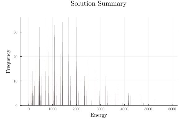
Let’s now solve this QUBO via traditional Integer Programming.
qubo_ilp_model = Model()

@variable(qubo_ilp_model, x_qubo_ilp[1:11], Bin, base_name = "x")
@variable(qubo_ilp_model, y[1:11, 1:11], Bin)

@objective(
    qubo_ilp_model,
    Min,
    sum(Q[i,j] * (i == j ? x_qubo_ilp[i] : y[i,j]) for i=1:11, j=1:11) +  β
)

@constraint(qubo_ilp_model, c1[i=1:11,j=1:11;i!=j], y[i,j] >= x_qubo_ilp[i] + x_qubo_ilp[j] - 1)
@constraint(qubo_ilp_model, c2[i=1:11,j=1:11;i!=j], y[i,j] <= x_qubo_ilp[i])
@constraint(qubo_ilp_model, c3[i=1:11,j=1:11;i!=j], y[i,j] <= x_qubo_ilp[j])

println(qubo_ilp_model)
Min -46 x[1] + 48 y[1,4] + 48 y[1,5] + 48 y[1,6] + 48 y[1,8] + 48 y[1,9] + 48 y[1,10] + 48 y[1,11] - 44 x[2] + 48 y[2,4] + 48 y[2,6] + 48 y[2,7] + 48 y[2,9] + 48 y[2,10] + 48 y[2,11] - 44 x[3] + 48 y[3,5] + 48 y[3,7] + 48 y[3,8] + 48 y[3,9] + 48 y[3,10] + 48 y[3,11] + 48 y[4,1] + 48 y[4,2] - 92 x[4] + 48 y[4,5] + 96 y[4,6] + 48 y[4,7] + 48 y[4,8] + 96 y[4,9] + [[...45 terms omitted...]] + 96 y[9,4] + 96 y[9,5] + 96 y[9,6] + 96 y[9,7] + 96 y[9,8] - 139 x[9] + 144 y[9,10] + 144 y[9,11] + 48 y[10,1] + 48 y[10,2] + 48 y[10,3] + 96 y[10,4] + 96 y[10,5] + 96 y[10,6] + 96 y[10,7] + 96 y[10,8] + 144 y[10,9] - 138 x[10] + 144 y[10,11] + 48 y[11,1] + 48 y[11,2] + 48 y[11,3] + 96 y[11,4] + 96 y[11,5] + 96 y[11,6] + 96 y[11,7] + 96 y[11,8] + 144 y[11,9] + 144 y[11,10] - 139 x[11] + 144
Subject to
c1[1,2] : -x[1] - x[2] + y[1,2] ≥ -1
 c1[1,3] : -x[1] - x[3] + y[1,3] ≥ -1
 c1[1,4] : -x[1] - x[4] + y[1,4] ≥ -1
 c1[1,5] : -x[1] - x[5] + y[1,5] ≥ -1
 c1[1,6] : -x[1] - x[6] + y[1,6] ≥ -1
 c1[1,7] : -x[1] - x[7] + y[1,7] ≥ -1
 c1[1,8] : -x[1] - x[8] + y[1,8] ≥ -1
 c1[1,9] : -x[1] - x[9] + y[1,9] ≥ -1
 c1[1,10] : -x[1] - x[10] + y[1,10] ≥ -1
 c1[1,11] : -x[1] - x[11] + y[1,11] ≥ -1
 c1[2,1] : -x[1] - x[2] + y[2,1] ≥ -1
 c1[2,3] : -x[2] - x[3] + y[2,3] ≥ -1
 c1[2,4] : -x[2] - x[4] + y[2,4] ≥ -1
 c1[2,5] : -x[2] - x[5] + y[2,5] ≥ -1
 c1[2,6] : -x[2] - x[6] + y[2,6] ≥ -1
 c1[2,7] : -x[2] - x[7] + y[2,7] ≥ -1
 c1[2,8] : -x[2] - x[8] + y[2,8] ≥ -1
 c1[2,9] : -x[2] - x[9] + y[2,9] ≥ -1
 c1[2,10] : -x[2] - x[10] + y[2,10] ≥ -1
 c1[2,11] : -x[2] - x[11] + y[2,11] ≥ -1
 c1[3,1] : -x[1] - x[3] + y[3,1] ≥ -1
 c1[3,2] : -x[2] - x[3] + y[3,2] ≥ -1
 c1[3,4] : -x[3] - x[4] + y[3,4] ≥ -1
 c1[3,5] : -x[3] - x[5] + y[3,5] ≥ -1
 c1[3,6] : -x[3] - x[6] + y[3,6] ≥ -1
 c1[3,7] : -x[3] - x[7] + y[3,7] ≥ -1
 c1[3,8] : -x[3] - x[8] + y[3,8] ≥ -1
 c1[3,9] : -x[3] - x[9] + y[3,9] ≥ -1
 c1[3,10] : -x[3] - x[10] + y[3,10] ≥ -1
 c1[3,11] : -x[3] - x[11] + y[3,11] ≥ -1
 c1[4,1] : -x[1] - x[4] + y[4,1] ≥ -1
 c1[4,2] : -x[2] - x[4] + y[4,2] ≥ -1
 c1[4,3] : -x[3] - x[4] + y[4,3] ≥ -1
 c1[4,5] : -x[4] - x[5] + y[4,5] ≥ -1
 c1[4,6] : -x[4] - x[6] + y[4,6] ≥ -1
 c1[4,7] : -x[4] - x[7] + y[4,7] ≥ -1
 c1[4,8] : -x[4] - x[8] + y[4,8] ≥ -1
 c1[4,9] : -x[4] - x[9] + y[4,9] ≥ -1
 c1[4,10] : -x[4] - x[10] + y[4,10] ≥ -1
 c1[4,11] : -x[4] - x[11] + y[4,11] ≥ -1
 c1[5,1] : -x[1] - x[5] + y[5,1] ≥ -1
 c1[5,2] : -x[2] - x[5] + y[5,2] ≥ -1
 c1[5,3] : -x[3] - x[5] + y[5,3] ≥ -1
 c1[5,4] : -x[4] - x[5] + y[5,4] ≥ -1
 c1[5,6] : -x[5] - x[6] + y[5,6] ≥ -1
 c1[5,7] : -x[5] - x[7] + y[5,7] ≥ -1
 c1[5,8] : -x[5] - x[8] + y[5,8] ≥ -1
 c1[5,9] : -x[5] - x[9] + y[5,9] ≥ -1
 c1[5,10] : -x[5] - x[10] + y[5,10] ≥ -1
 c1[5,11] : -x[5] - x[11] + y[5,11] ≥ -1
[[...362 constraints skipped...]]
 y[6,7] binary
 y[7,7] binary
 y[8,7] binary
 y[9,7] binary
 y[10,7] binary
 y[11,7] binary
 y[1,8] binary
 y[2,8] binary
 y[3,8] binary
 y[4,8] binary
 y[5,8] binary
 y[6,8] binary
 y[7,8] binary
 y[8,8] binary
 y[9,8] binary
 y[10,8] binary
 y[11,8] binary
 y[1,9] binary
 y[2,9] binary
 y[3,9] binary
 y[4,9] binary
 y[5,9] binary
 y[6,9] binary
 y[7,9] binary
 y[8,9] binary
 y[9,9] binary
 y[10,9] binary
 y[11,9] binary
 y[1,10] binary
 y[2,10] binary
 y[3,10] binary
 y[4,10] binary
 y[5,10] binary
 y[6,10] binary
 y[7,10] binary
 y[8,10] binary
 y[9,10] binary
 y[10,10] binary
 y[11,10] binary
 y[1,11] binary
 y[2,11] binary
 y[3,11] binary
 y[4,11] binary
 y[5,11] binary
 y[6,11] binary
 y[7,11] binary
 y[8,11] binary
 y[9,11] binary
 y[10,11] binary
 y[11,11] binary
set_optimizer(qubo_ilp_model, GLPK.Optimizer)

optimize!(qubo_ilp_model)

qubo_ilp_x = round.(Int, value.(x_qubo_ilp))

println(solution_summary(qubo_ilp_model))
println("* x = $qubo_ilp_x")
solution_summary(; result = 1, verbose = false)
├ solver_name : GLPK
├ Termination
│ ├ termination_status : OPTIMAL
│ ├ result_count : 1
│ ├ raw_status : Solution is optimal
│ └ objective_bound : 5.00000e+00
├ Solution (result = 1)
│ ├ primal_status : FEASIBLE_POINT
│ ├ dual_status : NO_SOLUTION
│ ├ objective_value : 5.00000e+00
│ └ relative_gap : 9.60000e+00
└ Work counters
└ solve_time (sec) : 7.99394e-03
* x = [0, 0, 0, 0, 0, 0, 0, 0, 1, 0, 0]
We observe that the optimal solution of this problem is otherwise, leading to an objective value of 5. Notice that this problem has a degenerate optimal solution given that otherwise also leads to the same solution.
Ising model
This section introduces the Ising model. We use JuMP to formulate Ising models and D-Wave’s neal to solve them with simulated annealing. For integer-programming comparisons, JuMP provides a common modeling interface to linear and nonlinear solvers. The examples use the open-source GLPK solver for mixed-integer linear programming.
Ising problem statement
We pose the Ising problem as the following optimization problem:
where we optimize over spins , on a constrained graph , where the quadratic coefficients are and the linear coefficients are . We also include an arbitrary offset of the Ising model .
h = [
    145.0,
    122.0,
    122.0,
    266.0,
    266.0,
    266.0,
    242.5,
    266.0,
    386.5,
    387.0,
    386.5,
]

J = [
    0  0  0 24 24 24  0 24 24 24 24
    0  0  0 24  0 24 24  0 24 24 24
    0  0  0  0 24  0 24 24 24 24 24
    0  0  0  0 24 48 24 24 48 48 48
    0  0  0  0  0 24 24 48 48 48 48
    0  0  0  0  0  0 24 24 48 48 48
    0  0  0  0  0  0  0 24 48 48 48
    0  0  0  0  0  0  0  0 48 48 48
    0  0  0  0  0  0  0  0  0 72 72
    0  0  0  0  0  0  0  0  0  0 72
    0  0  0  0  0  0  0  0  0  0  0
]

β = 1319.5

ising_model = Model()

@variable(ising_model, s[1:11], Spin)

@objective(ising_model, Min, s' * J * s + h' * s + β)

println(ising_model)
Min 24 s[4]*s[1] + 24 s[4]*s[2] + 24 s[5]*s[1] + 24 s[5]*s[3] + 24 s[5]*s[4] + 24 s[6]*s[1] + 24 s[6]*s[2] + 48 s[6]*s[4] + 24 s[6]*s[5] + 24 s[7]*s[2] + 24 s[7]*s[3] + 24 s[7]*s[4] + 24 s[7]*s[5] + 24 s[7]*s[6] + 24 s[8]*s[1] + 24 s[8]*s[3] + 24 s[8]*s[4] + 48 s[8]*s[5] + 24 s[8]*s[6] + 24 s[8]*s[7] + 24 s[9]*s[1] + 24 s[9]*s[2] + 24 s[9]*s[3] + 48 s[9]*s[4] + 48 s[9]*s[5] + 48 s[9]*s[6] + 48 s[9]*s[7] + 48 s[9]*s[8] + 24 s[10]*s[1] + 24 s[10]*s[2] + 24 s[10]*s[3] + 48 s[10]*s[4] + 48 s[10]*s[5] + 48 s[10]*s[6] + 48 s[10]*s[7] + 48 s[10]*s[8] + 72 s[10]*s[9] + 24 s[11]*s[1] + 24 s[11]*s[2] + 24 s[11]*s[3] + 48 s[11]*s[4] + 48 s[11]*s[5] + 48 s[11]*s[6] + 48 s[11]*s[7] + 48 s[11]*s[8] + 72 s[11]*s[9] + 72 s[11]*s[10] + 145 s[1] + 122 s[2] + 122 s[3] + 266 s[4] + 266 s[5] + 266 s[6] + 242.5 s[7] + 266 s[8] + 386.5 s[9] + 387 s[10] + 386.5 s[11] + 1319.5
Subject to
s[1] spin
 s[2] spin
 s[3] spin
 s[4] spin
 s[5] spin
 s[6] spin
 s[7] spin
 s[8] spin
 s[9] spin
 s[10] spin
 s[11] spin
set_optimizer(ising_model, ExactSampler.Optimizer)

optimize!(ising_model)

ising_s = round.(Int, value.(s))

# Display solution of the problem
println(solution_summary(ising_model))
println("* s = $ising_s")
solution_summary(; result = 1, verbose = false)
├ solver_name : Exact Sampler
├ Termination
│ ├ termination_status : LOCALLY_SOLVED
│ ├ result_count : 2048
│ └ raw_status : optimal
├ Solution (result = 1)
│ ├ primal_status : FEASIBLE_POINT
│ ├ dual_status : NO_SOLUTION
│ ├ objective_value : 5.00000e+00
│ └ dual_objective_value : 1.31950e+03
└ Work counters
└ solve_time (sec) : 8.50489e-04
* s = [-1, -1, -1, -1, -1, -1, -1, -1, 1, -1, -1]
plot(QUBOTools.EnergyFrequencyPlot(QUBOTools.solution(QUBOTools.backend(ising_model))))Before rebuilding the Ising model as a binary ILP, use the QUBOTools.qubo binary convention .
Under this substitution, the Ising Hamiltonian becomes a QUBO with a separate linear vector , a strictly off-diagonal quadratic matrix , and an offset . The scale and offset are already included in those returned pieces, so the ILP objective must include both the terms and the off-diagonal terms.
n, L, Q, α, β = QUBOTools.qubo(QUBOTools.backend(ising_model), :dense; sense = :min)QUBOTools.Form{Float64, QUBOTools.DenseLinearForm{Float64}, QUBOTools.DenseQuadraticForm{Float64}}(11, QUBOTools.DenseLinearForm{Float64}([-46.0, -44.0, -44.0, -92.0, -92.0, -92.0, -91.0, -92.0, -139.0, -138.0, -139.0]), QUBOTools.DenseQuadraticForm{Float64}([0.0 0.0 … 96.0 96.0; 0.0 0.0 … 96.0 96.0; … ; 0.0 0.0 … 0.0 288.0; 0.0 0.0 … 0.0 0.0]), 1.0, 144.0, QUBOTools.Frame(QUBOTools.Min, QUBOTools.BoolDomain))ising_ilp_model = Model()
@variable(ising_ilp_model, x_ising_ilp[1:n], Bin, base_name = "x")
@variable(ising_ilp_model, y[1:n, 1:n], Bin)
@objective(
ising_ilp_model,
Min,
sum(L[i] * x_ising_ilp[i] for i in 1:n) +
sum(Q[i,j] * y[i,j] for i in 1:n, j in 1:n if i != j) +
β
)
@constraint(ising_ilp_model, c1[i=1:n,j=1:n;i!=j], y[i,j] >= x_ising_ilp[i] + x_ising_ilp[j] - 1)
@constraint(ising_ilp_model, c2[i=1:n,j=1:n;i!=j], y[i,j] <= x_ising_ilp[i])
@constraint(ising_ilp_model, c3[i=1:n,j=1:n;i!=j], y[i,j] <= x_ising_ilp[j])
println(ising_ilp_model)Min -46 x[1] - 44 x[2] - 44 x[3] - 92 x[4] - 92 x[5] - 92 x[6] - 91 x[7] - 92 x[8] - 139 x[9] - 138 x[10] - 139 x[11] + 96 y[1,4] + 96 y[1,5] + 96 y[1,6] + 96 y[1,8] + 96 y[1,9] + 96 y[1,10] + 96 y[1,11] + 96 y[2,4] + 96 y[2,6] + 96 y[2,7] + 96 y[2,9] + 96 y[2,10] + 96 y[2,11] + 96 y[3,5] + 96 y[3,7] + 96 y[3,8] + 96 y[3,9] + 96 y[3,10] + 96 y[3,11] + 96 y[4,5] + 192 y[4,6] + 96 y[4,7] + 96 y[4,8] + 192 y[4,9] + 192 y[4,10] + 192 y[4,11] + 96 y[5,6] + 96 y[5,7] + 192 y[5,8] + 192 y[5,9] + 192 y[5,10] + 192 y[5,11] + 96 y[6,7] + 96 y[6,8] + 192 y[6,9] + 192 y[6,10] + 192 y[6,11] + 96 y[7,8] + 192 y[7,9] + 192 y[7,10] + 192 y[7,11] + 192 y[8,9] + 192 y[8,10] + 192 y[8,11] + 288 y[9,10] + 288 y[9,11] + 288 y[10,11] + 144
Subject to
c1[1,2] : -x[1] - x[2] + y[1,2] ≥ -1
c1[1,3] : -x[1] - x[3] + y[1,3] ≥ -1
c1[1,4] : -x[1] - x[4] + y[1,4] ≥ -1
c1[1,5] : -x[1] - x[5] + y[1,5] ≥ -1
c1[1,6] : -x[1] - x[6] + y[1,6] ≥ -1
c1[1,7] : -x[1] - x[7] + y[1,7] ≥ -1
c1[1,8] : -x[1] - x[8] + y[1,8] ≥ -1
c1[1,9] : -x[1] - x[9] + y[1,9] ≥ -1
c1[1,10] : -x[1] - x[10] + y[1,10] ≥ -1
c1[1,11] : -x[1] - x[11] + y[1,11] ≥ -1
c1[2,1] : -x[1] - x[2] + y[2,1] ≥ -1
c1[2,3] : -x[2] - x[3] + y[2,3] ≥ -1
c1[2,4] : -x[2] - x[4] + y[2,4] ≥ -1
c1[2,5] : -x[2] - x[5] + y[2,5] ≥ -1
c1[2,6] : -x[2] - x[6] + y[2,6] ≥ -1
c1[2,7] : -x[2] - x[7] + y[2,7] ≥ -1
c1[2,8] : -x[2] - x[8] + y[2,8] ≥ -1
c1[2,9] : -x[2] - x[9] + y[2,9] ≥ -1
c1[2,10] : -x[2] - x[10] + y[2,10] ≥ -1
c1[2,11] : -x[2] - x[11] + y[2,11] ≥ -1
c1[3,1] : -x[1] - x[3] + y[3,1] ≥ -1
c1[3,2] : -x[2] - x[3] + y[3,2] ≥ -1
c1[3,4] : -x[3] - x[4] + y[3,4] ≥ -1
c1[3,5] : -x[3] - x[5] + y[3,5] ≥ -1
c1[3,6] : -x[3] - x[6] + y[3,6] ≥ -1
c1[3,7] : -x[3] - x[7] + y[3,7] ≥ -1
c1[3,8] : -x[3] - x[8] + y[3,8] ≥ -1
c1[3,9] : -x[3] - x[9] + y[3,9] ≥ -1
c1[3,10] : -x[3] - x[10] + y[3,10] ≥ -1
c1[3,11] : -x[3] - x[11] + y[3,11] ≥ -1
c1[4,1] : -x[1] - x[4] + y[4,1] ≥ -1
c1[4,2] : -x[2] - x[4] + y[4,2] ≥ -1
c1[4,3] : -x[3] - x[4] + y[4,3] ≥ -1
c1[4,5] : -x[4] - x[5] + y[4,5] ≥ -1
c1[4,6] : -x[4] - x[6] + y[4,6] ≥ -1
c1[4,7] : -x[4] - x[7] + y[4,7] ≥ -1
c1[4,8] : -x[4] - x[8] + y[4,8] ≥ -1
c1[4,9] : -x[4] - x[9] + y[4,9] ≥ -1
c1[4,10] : -x[4] - x[10] + y[4,10] ≥ -1
c1[4,11] : -x[4] - x[11] + y[4,11] ≥ -1
c1[5,1] : -x[1] - x[5] + y[5,1] ≥ -1
c1[5,2] : -x[2] - x[5] + y[5,2] ≥ -1
c1[5,3] : -x[3] - x[5] + y[5,3] ≥ -1
c1[5,4] : -x[4] - x[5] + y[5,4] ≥ -1
c1[5,6] : -x[5] - x[6] + y[5,6] ≥ -1
c1[5,7] : -x[5] - x[7] + y[5,7] ≥ -1
c1[5,8] : -x[5] - x[8] + y[5,8] ≥ -1
c1[5,9] : -x[5] - x[9] + y[5,9] ≥ -1
c1[5,10] : -x[5] - x[10] + y[5,10] ≥ -1
c1[5,11] : -x[5] - x[11] + y[5,11] ≥ -1
[[...362 constraints skipped...]]
y[6,7] binary
y[7,7] binary
y[8,7] binary
y[9,7] binary
y[10,7] binary
y[11,7] binary
y[1,8] binary
y[2,8] binary
y[3,8] binary
y[4,8] binary
y[5,8] binary
y[6,8] binary
y[7,8] binary
y[8,8] binary
y[9,8] binary
y[10,8] binary
y[11,8] binary
y[1,9] binary
y[2,9] binary
y[3,9] binary
y[4,9] binary
y[5,9] binary
y[6,9] binary
y[7,9] binary
y[8,9] binary
y[9,9] binary
y[10,9] binary
y[11,9] binary
y[1,10] binary
y[2,10] binary
y[3,10] binary
y[4,10] binary
y[5,10] binary
y[6,10] binary
y[7,10] binary
y[8,10] binary
y[9,10] binary
y[10,10] binary
y[11,10] binary
y[1,11] binary
y[2,11] binary
y[3,11] binary
y[4,11] binary
y[5,11] binary
y[6,11] binary
y[7,11] binary
y[8,11] binary
y[9,11] binary
y[10,11] binary
y[11,11] binary
set_optimizer(ising_ilp_model, GLPK.Optimizer)

optimize!(ising_ilp_model)

ising_ilp_x = round.(Int, value.(x_ising_ilp))
ising_ilp_s = 2 .* ising_ilp_x .- 1

@assert ising_ilp_s == ising_s
@assert isapprox(objective_value(ising_ilp_model), objective_value(ising_model); atol = 1e-6)

println(solution_summary(ising_ilp_model))
println("* x = $ising_ilp_x")
println("* s = $ising_ilp_s")
solution_summary(; result = 1, verbose = false)
├ solver_name : GLPK
├ Termination
│ ├ termination_status : OPTIMAL
│ ├ result_count : 1
│ ├ raw_status : Solution is optimal
│ └ objective_bound : 5.00000e+00
├ Solution (result = 1)
│ ├ primal_status : FEASIBLE_POINT
│ ├ dual_status : NO_SOLUTION
│ ├ objective_value : 5.00000e+00
│ └ relative_gap : 7.40000e+00
└ Work counters
└ solve_time (sec) : 3.16906e-03
* x = [0, 0, 0, 0, 0, 0, 0, 0, 1, 0, 0]
* s = [-1, -1, -1, -1, -1, -1, -1, -1, 1, -1, -1]
The corrected ILP solution is , which maps back to through . This matches the ExactSampler solution and gives objective value 5.0.
From QUBO to Ising
QUBO and Ising models describe the same binary search space with different variable conventions. The QUBO form uses variables in {0, 1}, while the Ising form uses spins in {-1, +1}. Moving between them changes the linear terms, quadratic terms, and offset, but not the underlying set of assignments. This equivalence lets us compare exact integer-programming solves with simulated annealing on the same problem.
Let’s now solve the QUBO problem using Simulated Annealing
set_optimizer(qubo_model, DWave.Neal.Optimizer)

set_optimizer_attribute(qubo_model, "num_reads", 1_000)

optimize!(qubo_model)

qubo_x = round.(Int, value.(x_qubo))

println(solution_summary(qubo_model))
println("* x = $qubo_x")
solution_summary(; result = 1, verbose = false)
├ solver_name : D-Wave Neal Simulated Annealing Sampler
├ Termination
│ ├ termination_status : LOCALLY_SOLVED
│ ├ result_count : 9
│ └ raw_status : locally_solved
├ Solution (result = 1)
│ ├ primal_status : FEASIBLE_POINT
│ ├ dual_status : NO_SOLUTION
│ ├ objective_value : 5.00000e+00
│ └ dual_objective_value : 1.44000e+02
└ Work counters
└ solve_time (sec) : 6.40306e-01
* x = [0, 0, 0, 0, 0, 0, 0, 0, 0, 0, 1]
plot(QUBOTools.EnergyFrequencyPlot(QUBOTools.solution(QUBOTools.backend(qubo_model))))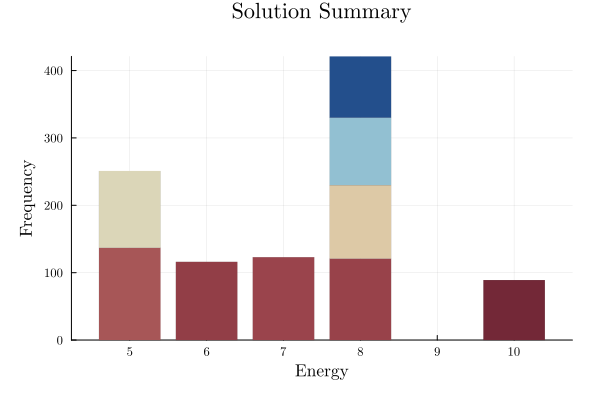
Notice that this is the same example we have been solving earlier (via Integer Programming in the Quiz 1 and Ising model above).
From penalty models to graph coloring
The previous examples used penalties to enforce algebraic constraints. Graph coloring uses the same idea with one-hot variables: each vertex must choose exactly one color, and adjacent vertices may not share a color. Violating either rule adds a penalty to the QUBO objective, so low-energy samples correspond to valid colorings when the penalties are large enough.
Let’s solve the graph coloring problem using QUBO.
Vertex -coloring of graphs
Given a graph , where is the set of vertices and is the set of edges of , and a positive integer , we ask if it is possible to assign a color to every vertex from , such that adjacent vertices have different colors assigned.
has 12 vertices and 23 edges. We ask if the graph is 3–colorable. Let’s first encode and using Julia data structures:
Note: This second tutorial is heavily inspired in D-Wave’s Map coloring of Canada found here.
V = 1:12
E = [
    (1,2), (1,4), (1,6), (1,12),
    (2,3), (2,5), (2,7),
    (3,8), (3,10),
    (4,9), (4,11),
    (5,6), (5,9), (5,12),
    (6,7), (6,10),
    (7,8), (7,11),
    (8,9), (8,12),
    (9,10),
    (10,11),
    (11,12),
]

G = SimpleGraph(Edge.(E))
{12, 23} undirected simple Int64 graphgraph_layout = Vector{Point}(undef, 12)
graph_layout[1] = Point(-1.5,-1.5)
graph_layout[2] = Point(1.5,-1.5)
graph_layout[3] = Point(1.5,1.5)
graph_layout[4] = Point(-1.5,1.5)
for i in 5:12
graph_layout[i] = Point(cos((2i+1) * π/8), -sin((2i+1) * π/8))
end
@drawsvg(
begin
sethue("black")
background("white")
drawgraph(
G;
layout=100 * graph_layout,
vertexlabels = V,
)
end,
)# Valid configurations for the constraint that each node select a single color, in this case we want to use 3 colors
color_model = direct_model(ToQUBO.Optimizer(DWave.Neal.Optimizer))
@variable(color_model, c[1:12,1:3], Bin)
# Each node must be colored with exactly one color
@constraint(color_model, unique[i=1:12], sum(c[i,:]) == 1)
# Add constraint that each pair of nodes with a shared edge not both select one color
@constraint(color_model, neigh[(i,j) ∈ E, k=1:3], c[i, k] * c[j,k] == 0);optimize!(color_model)
color_ρ = get_optimizer_attribute.(neigh, ToQUBO.Attributes.ConstraintEncodingPenalty())
color_c = round.(Int, value.(c))
println(solution_summary(color_model))
println("* c = $color_c")
println("* ρ = $color_ρ")solution_summary(; result = 1, verbose = false)
├ solver_name : Virtual QUBO Model
├ Termination
│ ├ termination_status : LOCALLY_SOLVED
│ ├ result_count : 170
│ └ raw_status : locally_solved
├ Solution (result = 1)
│ ├ primal_status : FEASIBLE_POINT
│ ├ dual_status : NO_SOLUTION
│ └ objective_value : 0.00000e+00
└ Work counters
└ solve_time (sec) : 5.64137e-01
* c = [0 1 0; 1 0 0; 0 0 1; 0 0 1; 0 1 0; 1 0 0; 0 0 1; 0 1 0; 1 0 0; 0 1 0; 1 0 0; 0 0 1]
* ρ = 2-dimensional DenseAxisArray{Float64,2,...} with index sets:
Dimension 1, [(1, 2), (1, 4), (1, 6), (1, 12), (2, 3), (2, 5), (2, 7), (3, 8), (3, 10), (4, 9) … (5, 12), (6, 7), (6, 10), (7, 8), (7, 11), (8, 9), (8, 12), (9, 10), (10, 11), (11, 12)]
Dimension 2, Base.OneTo(3)
And data, a 23×3 Matrix{Float64}:
1.0 1.0 1.0
1.0 1.0 1.0
1.0 1.0 1.0
1.0 1.0 1.0
1.0 1.0 1.0
1.0 1.0 1.0
1.0 1.0 1.0
1.0 1.0 1.0
1.0 1.0 1.0
1.0 1.0 1.0
1.0 1.0 1.0
1.0 1.0 1.0
1.0 1.0 1.0
1.0 1.0 1.0
1.0 1.0 1.0
1.0 1.0 1.0
1.0 1.0 1.0
1.0 1.0 1.0
1.0 1.0 1.0
1.0 1.0 1.0
1.0 1.0 1.0
1.0 1.0 1.0
1.0 1.0 1.0
QUBOTools.EnergyFrequencyPlot(QUBOTools.solution(JuMP.backend(color_model).optimizer)) |> plot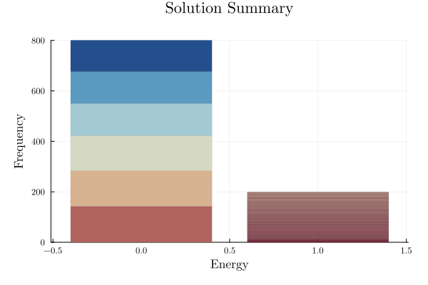
@drawsvg(
    begin
        sethue("black")
        background("white")
        drawgraph(
            G;
            layout=100 * graph_layout,
            vertexlabels = V,
            vertexfillcolors = (v) -> begin
                if color_c[v,1] > 0
                    return colorant"red"
                elseif color_c[v,2] > 0
                    return colorant"blue"
                elseif color_c[v,3] > 0
                    return colorant"green"
                else
                    return colorant"white"
                end
            end
        )
    end,
)Practice checkpoints
Use these checkpoints during the workshop to test the main ideas before moving on.
# =============================================================================
# EXERCISE 1: Build a small QUBO by hand
# =============================================================================
# Write the QUBO coefficients for a three-variable penalty model before using any helper function. Check that the lowest-energy assignment satisfies the original constraint.
#
# Hint: Enumerate all eight assignments to validate the coefficients.
#
# Your code here:
# =============================================================================
Notebook Cell
# SOLUTION (hidden in workshop version):
# Build and enumerate a three-variable one-hot QUBO by hand.
assignments = vec(collect(Iterators.product(0:1, 0:1, 0:1)))
linear = [-1.0, -1.0, -1.0]
quadratic = Dict((1, 2) => 2.0, (1, 3) => 2.0, (2, 3) => 2.0)
function energy(bits)
    total = 1.0
    for i in 1:3
        total += linear[i] * bits[i]
    end
    for (edge, weight) in quadratic
        i, j = edge
        total += weight * bits[i] * bits[j]
    end
    return total
end
best = sort(
    [(Tuple(bits), energy(bits)) for bits in assignments];
    by = item -> (item[2], -item[1][1], -item[1][2], -item[1][3]),
)[1]
feasible = sum(collect(best[1])) == 1
println("best_assignment = $(best[1]); energy = $(best[2]); feasible = $(feasible)")
best_assignment = (1, 0, 0); energy = 0.0; feasible = true
# =============================================================================
# EXERCISE 2: Stress-test the penalty parameter
# =============================================================================
# Lower rho below the sufficient bound and sample or enumerate the resulting BQM. Record the first infeasible assignment that becomes competitive with a feasible one.
#
# Hint: Keep the objective and constraints fixed so rho is the only changed input.
#
# Your code here:
# =============================================================================
Notebook Cell
# SOLUTION (hidden in workshop version):
# Lower rho on a tiny equality-constrained binary model and detect infeasibility.
assignments = vec(collect(Iterators.product(0:1, 0:1, 0:1)))
A_small = [1 1 0; 0 1 1]
b_small = [1, 1]
c_small = [1.0, 2.0, 1.0]
penalized_energy(bits, rho_value) = begin
    x = collect(bits)
    residual = A_small * x - b_small
    c_small' * x + rho_value * (residual' * residual)
end
rho_value = 0.25
best = sort([(Tuple(bits), penalized_energy(bits, rho_value), A_small * collect(bits) == b_small) for bits in assignments]; by = item -> item[2])[1]
println("rho = $(rho_value); best_assignment = $(best[1]); energy = $(best[2]); feasible = $(best[3])")
rho = 0.25; best_assignment = (0, 0, 0); energy = 0.5; feasible = false
# =============================================================================
# EXERCISE 3: Extend graph coloring
# =============================================================================
# Change the graph-coloring example to use three colors. Update the variable naming and validity checks so exactly one color is assigned per node.
#
# Hint: The exactly-one penalties scale with the number of colors, not the number of nodes.
#
# Your code here:
# =============================================================================
Notebook Cell
# SOLUTION (hidden in workshop version):
# Create variables and constraints for a three-color graph-coloring BQM sketch.
nodes = 1:3
edges = [(1, 2), (2, 3)]
colors = ["red", "green", "blue"]
variables = Dict((node, color) => "x_$(node)_$(color)" for node in nodes for color in colors)
one_hot_groups = [[variables[(node, color)] for color in colors] for node in nodes]
edge_conflicts = [(variables[(u, color)], variables[(v, color)]) for (u, v) in edges for color in colors]
format_group(group) = join(group, ",")
format_conflict(conflict) = "$(conflict[1])-$(conflict[2])"
formatted_groups = join(format_group.(one_hot_groups), " | ")
formatted_conflicts = join(format_conflict.(edge_conflicts), " | ")
println("one_hot_groups = $(formatted_groups); edge_conflicts = $(formatted_conflicts)")
one_hot_groups = x_1_red,x_1_green,x_1_blue | x_2_red,x_2_green,x_2_blue | x_3_red,x_3_green,x_3_blue; edge_conflicts = x_1_red-x_2_red | x_1_green-x_2_green | x_1_blue-x_2_blue | x_2_red-x_3_red | x_2_green-x_3_green | x_2_blue-x_3_blue
Summary
In this notebook we:
Defined QUBO and Ising objectives and identified how coefficients encode binary optimization problems.
Reformulated constrained binary problems with penalty terms so they can be sampled as unconstrained models.
Used JuliaQUBO tooling and simulated annealing to solve models and inspect sampled energies.
Modeled graph coloring directly from penalties and validated feasible color assignments.
Learning objectives met: You practiced reading QUBO/Ising forms, building QUBO models, applying penalty reformulations, and checking sampled solutions against the original constraints.
Next steps: Proceed to Notebook 3: GAMA to compare QUBO-style sampling with Graver-basis augmentation for structured integer programs.
Further reading:
References
David E. Bernal Neira — Davidson School of Chemical Engineering, Purdue University
Pedro Maciel Xavier — Davidson School of Chemical Engineering, Purdue University
João Victor Souza — Computer Engineering Department, Military Institute of Engineering (IME)
Acknowledgments
This notebook was developed by: