Benchmarking (Python) - QUBONotebooks: Quantum Integer Programming

Maintained by the JuliaQUBO organization
SECQUOIA · PSR Energy

Setup¶

Google Colab¶

Click the badge above to open this notebook in Colab. The notebook installs or activates dependencies in the setup cells below.

Local installation¶

Run the following from the repository root before opening this notebook locally:

python -m pip install dimod dwave-neal matplotlib networkx numpy pandas pyomo scipy tqdm

The bundled cache avoids the long benchmark regeneration cells.

Learning objectives¶

By the end of this notebook you will be able to:

Define solver, instance, schedule, and hyperparameter ensembles for benchmarking experiments.
Compute and interpret time-to-solution, success probability, and performance-ratio summaries.
Use bootstrap summaries to compare solver settings across repeated samples and instance ensembles.
Explain the difference between default, tuned, ensemble-selected, and virtual-best parameter choices.

Prerequisites¶

Mathematical background: QUBO/Ising models, probability, medians, and confidence intervals.
Prior notebooks: Notebooks 2-4, especially QUBO construction and simulated/quantum annealing outputs.
Accounts required: None for the bundled cache; regenerating hardware data may require solver access.
Python version: Python 3.9+ with the repository’s benchmarking dependencies.

About this notebook¶

A solver is the combination of hardware, algorithm, software, parameter settings, and resource limits used to solve an optimization problem. No configuration is best for every problem family or computational budget.

Tuning every parameter on the target instance consumes the same time, memory, or energy budget that the final solve is meant to conserve, and it can overfit one instance. A more realistic workflow tunes configurations offline on a representative family of training instances, then evaluates the selected configuration on held-out or previously unseen instances.

This notebook develops metrics and experiments for comparing solver configurations across repeated samples and related problem instances.

Benchmarking example¶

For illustration purposes, we will use an example that you are already familiar with, which is an Ising model. As a solver, we will use a simulated annealing code provided by D-Wave Ocean Tools.

Ising model¶

We use D-Wave’s dimod and neal packages to define Ising models and solve them with simulated annealing.

Ising problem statement¶

We pose the Ising problem as the following optimization problem:

\min_{s \in \{ \pm 1 \}^n} H(s) = \min_{s \in \{ \pm 1 \}^n} \sum_{(i, j) \in E(G)} J_{i,j}s_is_j + \sum_{i \in V(G)} h_is_i + \beta

(1)

where we optimize over spins $s \in \{ \pm 1 \}^n$ , on a constrained graph $G(V,E)$ , where the quadratic coefficients are $J_{i,j}$ and the linear coefficients are $h_i$ . We also include an arbitrary offset of the Ising model $\beta$ .

Small Ising example¶

Suppose we have an Ising model defined from

h = \begin{bmatrix} 145.0 \\ 122.0 \\ 122.0 \\ 266.0 \\ 266.0 \\ 266.0 \\ 242.5 \\ 266.0 \\ 386.5 \\ 387.0 \\ 386.5 \end{bmatrix}, J = \begin{bmatrix} 0 & 0 & 0 & 24 & 24 & 24 & 24 & 24 & 24 & 24 & 24\\ 0 & 0 & 0 & 24 & 0 & 24 & 24 & 24 & 24 & 24 & 24\\ 0 & 0 & 0 & 0 & 24 & 0 & 24 & 24 & 24 & 24 & 24\\ 0 & 0 & 0 & 0 & 24 & 48 & 24 & 24 & 48 & 48 & 48\\ 0 & 0 & 0 & 0 & 0 & 24 & 24 & 48 & 48 & 48 & 48\\ 0 & 0 & 0 & 0 & 0 & 0 & 24 & 24 & 48 & 48 & 48\\ 0 & 0 & 0 & 0 & 0 & 0 & 0 & 24 & 48 & 48 & 48\\ 0 & 0 & 0 & 0 & 0 & 0 & 0 & 0 & 48 & 48 & 48\\ 0 & 0 & 0 & 0 & 0 & 0 & 0 & 0 & 0 & 72 & 72\\ 0 & 0 & 0 & 0 & 0 & 0 & 0 & 0 & 0 & 0 & 72\\ 0 & 0 & 0 & 0 & 0 & 0 & 0 & 0 & 0 & 0 & 0\\ \end{bmatrix} \text{ and } c_I = 1319.5

(2)

Let’s solve this problem

# If using this on Google Colab, we need to install the packages
try:
  import google.colab
  IN_COLAB = True
except:
  IN_COLAB = False

# Install the packages used by this notebook
if IN_COLAB:
    !pip install -q pyomo dimod dwave-neal scipy pandas networkx matplotlib tqdm

# Import the Pyomo library, which can be installed via pip, conda, or from GitHub: https://github.com/Pyomo/pyomo
import pyomo.environ as pyo
# Import the Dwave packages dimod and neal
import dimod
import neal
# Import Matplotlib to generate plots
import matplotlib.pyplot as plt
# Import numpy and scipy for certain numerical calculations below
import numpy as np
import math
from collections import Counter
import pandas as pd
from itertools import chain
import time
import networkx as nx
import os
import pickle
from scipy import stats
from matplotlib import ticker

try:
    from tqdm.auto import tqdm
except ImportError:
    def tqdm(iterable, **kwargs):
        return iterable

<python-environment>/lib/python3.12/site-packages/tqdm/auto.py:21: TqdmWarning: IProgress not found. Please update jupyter and ipywidgets. See https://ipywidgets.readthedocs.io/en/stable/user_install.html
  from .autonotebook import tqdm as notebook_tqdm

# These could also be simple lists and numpy matrices
h = {0: 145.0, 1: 122.0, 2: 122.0, 3: 266.0, 4: 266.0, 5: 266.0, 6: 242.5, 7: 266.0, 8: 386.5, 9: 387.0, 10: 386.5}
J = {(0, 3): 24.0, (0, 4): 24.0, (0, 5): 24.0, (0, 7): 24.0, (0, 8): 24.0, (0, 9): 24.0, (0, 10): 24.0, (1, 3): 24.0, (1, 5): 24.0, (1, 6): 24.0, (1, 8): 24.0, (1, 9): 24.0, (1, 10): 24.0, (2, 4): 24.0, (2, 6): 24.0, (2, 7): 24.0, (2, 8): 24.0, (2, 9): 24.0, (2, 10): 24.0, (3, 4): 24.0, (3, 5): 48.0, (3, 6): 24.0, (3, 7): 24.0, (3, 8): 48.0, (3, 9): 48.0, (3, 10): 48.0, (4, 5): 24.0, (4, 6): 24.0, (4, 7): 48.0, (4, 8): 48.0, (4, 9): 48.0, (4, 10): 48.0, (5, 6): 24.0, (5, 7): 24.0, (5, 8): 48.0, (5, 9): 48.0, (5, 10): 48.0, (6, 7): 24.0, (6, 8): 48.0, (6, 9): 48.0, (6, 10): 48.0, (7, 8): 48.0, (7, 9): 48.0, (7, 10): 48.0, (8, 9): 72.0, (8, 10): 72.0, (9, 10): 72.0}
cI = 1319.5


model_ising = dimod.BinaryQuadraticModel.from_ising(h, J, offset=cI) # define the model

nx_graph = dimod.to_networkx_graph(model_ising)
edges, bias = zip(*nx.get_edge_attributes(nx_graph, 'bias').items())
bias = np.array(bias)
nx.draw(nx_graph, node_size=15, pos=nx.spring_layout(nx_graph, seed=314159),
        edgelist=edges, edge_color=bias, edge_cmap=plt.cm.Blues)

Since the problem is relatively small (11 variables, $2^{11}=2048$ combinations), we can afford to enumerate all the solutions.

exactSampler = dimod.reference.samplers.ExactSolver()
start = time.time()
exactSamples = exactSampler.sample(model_ising)
timeEnum = time.time() - start
print("runtime: " + str(timeEnum) + " seconds")

runtime: 0.001972198486328125 seconds

# Some useful functions to get plots
def plot_energy_values(results, title=None):

    _, ax = plt.subplots()

    energies = [datum.energy for datum in results.data(
        ['energy'], sorted_by='energy')]

    if results.vartype == dimod.BINARY:
        samples = [''.join(c for c in str(datum.sample.values()).strip(
            ', ') if c.isdigit()) for datum in results.data(['sample'], sorted_by=None)]
        ax.set(xlabel='bitstring for solution')
    else:
        samples = np.arange(len(energies))
        ax.set(xlabel='solution')

    ax.bar(samples, energies)
    ax.tick_params(axis='x', rotation=90)
    ax.set_ylabel('Energy')
    if title:
        ax.set_title(str(title))
    print("minimum energy:", min(energies))
    return ax


def plot_samples(results, title=None, skip=1):
    _, ax = plt.subplots()

    energies = [datum.energy for datum in results.data(
        ['energy'], sorted_by='energy')]

    if results.vartype == dimod.BINARY:
        samples = [''.join(c for c in str(datum.sample.values()).strip(
            ', ') if c.isdigit()) for datum in results.data(['sample'], sorted_by=None)]
        ax.set_xlabel('bitstring for solution')
    else:
        samples = np.arange(len(energies))
        ax.set_xlabel('solution')

    counts = Counter(samples)
    total = len(samples)
    for key in counts:
        counts[key] /= total
    df = pd.DataFrame.from_dict(counts, orient='index').sort_index()
    df.plot(kind='bar', legend=None, ax=ax)

    ax.tick_params(axis='x', rotation=80)
    ax.set_xticklabels([t.get_text()[:7] if not i%skip else "" for i,t in enumerate(ax.get_xticklabels())])
    ax.set_ylabel('Probabilities')
    if title:
        ax.set_title(str(title))
    print("minimum energy:", min(energies))
    return ax


def plot_energy_cfd(results, title=None, skip=1):
    _, ax = plt.subplots()
    # skip parameter given to avoid putting all xlabels
    energies = results.data_vectors['energy']
    occurrences = results.data_vectors['num_occurrences']
    counts = Counter(energies)
    total = sum(occurrences)
    counts = {}
    for index, energy in enumerate(energies):
        if energy in counts.keys():
            counts[energy] += occurrences[index]
        else:
            counts[energy] = occurrences[index]
    for key in counts:
        counts[key] /= total
    df = pd.DataFrame.from_dict(counts, orient='index').sort_index()
    df.plot(kind='bar', legend=None, ax = ax)
    ax.set_xticklabels([t.get_text()[:7] if not i%skip else "" for i,t in enumerate(ax.get_xticklabels())])

    ax.set_xlabel('Energy')
    ax.set_ylabel('Probabilities')
    if title:
        ax.set_title(str(title))
    print("minimum energy:", min(energies))
    return ax

plot_energy_values(exactSamples, title='Enumerate all solutions')
plot_energy_cfd(exactSamples, title='Enumerate all solutions', skip=10)

minimum energy: 5.0
minimum energy: 5.0

<Axes: title={'center': 'Enumerate all solutions'}, xlabel='Energy', ylabel='Probabilities'>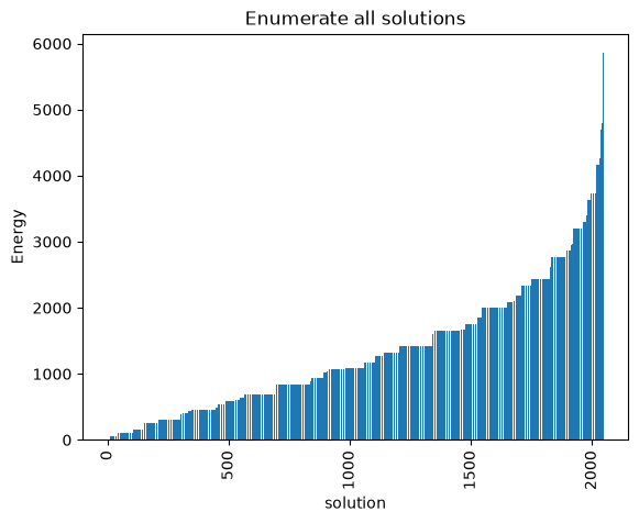

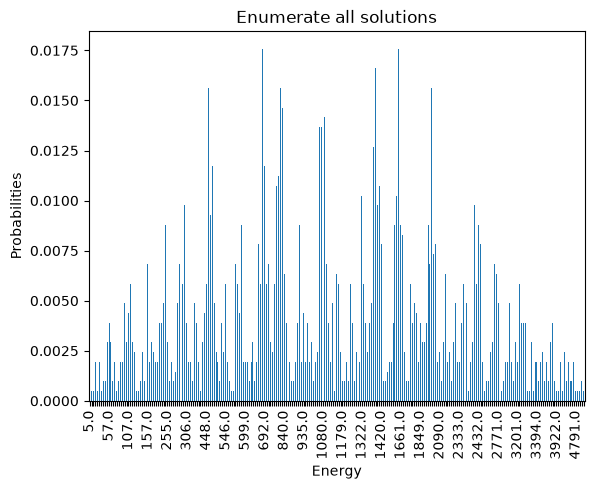
We observe that the optimal solution of this problem is $x_{10} = 1, 0$ otherwise, leading to an objective of 5. Notice that this problem has a degenerate optimal solution given that $x_8 = 1, 0$ otherwise also leads to the same solution.

Let’s now solve this problem using Simulated Annealing

Simulated Annealing (SA)¶

SA is an optimization algorithm that works by navigating the input space and evaluating the objective function (energy) similarly to hill climbing. The main difference is that SA implements a strategy to avoid getting stuck in local optima.

The general idea is to allow moves to a worse position, but in a structured way. When a candidate solution is selected, the probability of actually moving to the new position is determined by the change in the objective function and by a metric called temperature. When the temperature is high, the chance of performing a jump to a worse state increases, and the opposite happens when the temperature is low. By continuously decreasing the temperature during the execution of the algorithm, it can escape local optima during the first stages (high temperature), but it settles into a position towards the end of the execution (low temperature).

Probability of Making a Jump¶

Case 1:

\Delta E = E_{current} - E_{next} > 0

(3)

It is always advantageous to move to a state with a better objective function. In this case, the probability is $P = 1$ .

Case 2:

\Delta E = E_{current} - E_{next} < 0

(4)

In this case, the probability of taking the step is determined by:

P = e^{-|\Delta E| / T}

(5)

Note: This formulation applies to a minimization problem. To solve a maximization problem, the only change is that $\Delta E = E_{next} - E_{current}$ .

Temperature Decrease¶

The way the temperature decreases during the algorithm’s execution varies between implementations. This is referred to as the temperature schedule, which is a function of time or the number of iterations.

Note: $\beta = 1 / T$ is also commonly used in the implementation of the algorithm.

simAnnSampler = neal.SimulatedAnnealingSampler()
simAnnSamples = simAnnSampler.sample(model_ising, seed=314159, num_reads=1000)

plot_energy_values(simAnnSamples, title='Simulated annealing in default parameters')
plot_energy_cfd(simAnnSamples, title='Simulated annealing in default parameters')

minimum energy: 5.0
minimum energy: 5.0

<Axes: title={'center': 'Simulated annealing in default parameters'}, xlabel='Energy', ylabel='Probabilities'>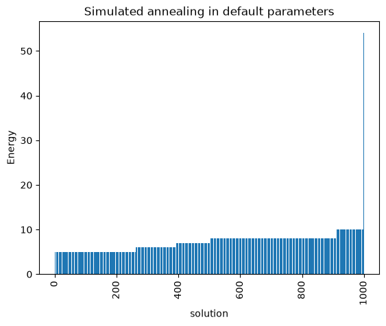

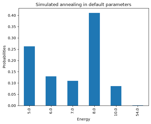
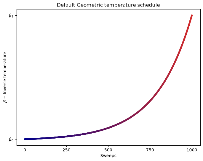
We are going to use the default limits of temperature given by the simulating annealing code. These are defined using the minimum and maximum nonzero coefficients in the Ising model. Then the range for beta is defined as

\beta \in \left[ \frac{\log(2)}{\max \{ \Delta E \} },\frac{\log(100)}{\min \{ \Delta E \} } \right]

(6)

where

\Delta E = \min_{i} \{h_i \} + \sum_j J_{ij}+J_{ji}

(7)

Hot temperature: We want to scale hot_beta so that for the most unlikely qubit flip, we get at least 50% chance of flipping. (This means all other qubits will have > 50% chance of flipping initially). Most unlikely flip is when we go from a very low energy state to a high energy state, thus we calculate hot_beta based on max_delta_energy.

0.50 = \exp(-\overline{\beta} * \max \{ \Delta E \})

(8)

Cold temperature: Towards the end of the annealing schedule, we want to minimize the chance of flipping. Don’t want to be stuck between small energy tweaks. Hence, set cold_beta so that at minimum energy change, the chance of flipping is set to 1%.

0.01 = \exp(-\underline{\beta} * \min \{ \Delta E \})

(9)

By default, the schedule also follows a geometric series.

def geomspace(a, b, length=100):
    return np.logspace(np.log10(a), np.log10(b), num=length, endpoint=True)

def hex_to_RGB(hex_str):
    return [int(hex_str[i:i+2], 16) for i in range(1,6,2)]

def get_color_gradient(c1, c2, n):
    assert n > 1
    c1_rgb = np.array(hex_to_RGB(c1))/255
    c2_rgb = np.array(hex_to_RGB(c2))/255
    mix_pcts = [x/(n-1) for x in range(n)]
    rgb_colors = [((1-mix)*c1_rgb + (mix*c2_rgb)) for mix in mix_pcts]
    return ["#" + "".join([format(int(round(val*255)), "02x") for val in item]) for item in rgb_colors]

def plot_schedule(beta1, beta2, length=1000):
    color1 = "#00008b"
    color2 = "#D22B2B"
    sweeps = np.linspace(np.log10(2), np.log10(100), num=length, endpoint=True)
    beta = np.geomspace(beta1, beta2, num=length)
    plt.figure(figsize=(8, 6))
    plt.scatter(x=sweeps, 
                y=beta, 
                color = get_color_gradient(color1, color2, len(beta)), 
                s=10)
    plt.title("Default Geometric temperature schedule")
    plt.xlabel("Sweeps")
    plt.ylabel(r"$ \beta $ = Inverse temperature")
    plt.xticks([sweeps[0], sweeps[249], sweeps[499], sweeps[749], sweeps[999]], [0,250,500,750,1000])
    plt.yticks([beta1, beta2], [r"$ \beta_{0} $", r"$ \beta_{1} $"])
    plt.grid(False)
    plt.show()

beta1 = 0.1
beta2 = 10
plot_schedule(beta1, beta2)

Now let’s compute an expected time metric with respect to the number of sweeps in simulated annealing.

s = 0.99
# sweeps = list(chain(np.arange(1,10,1),np.arange(10,30,2), np.arange(30,50,5), np.arange(50,100,10) ,np.arange(100,1001,100)))
sweeps = list(chain(np.arange(1, 250, 1), np.arange(250, 1001, 10)))
schedules = ['geometric','linear']
opt_energy = 5
results = {}
results['p'] = {}
results['tts'] = {}
results['t']= {}
for schedule in schedules:
    probs = []
    time_to_sol = []
    times = []
    for sweep in sweeps:
        start = time.time()
        samples = simAnnSampler.sample(model_ising, seed=314159, num_reads=1000, num_sweeps=sweep, beta_schedule_type=schedule)
        time_s = time.time() - start
        energies=samples.data_vectors['energy']
        occurrences = samples.data_vectors['num_occurrences']
        total_counts = sum(occurrences)
        counts = {}
        for index, energy in enumerate(energies):
            if energy in counts.keys():
                counts[energy] += occurrences[index]
            else:
                counts[energy] = occurrences[index]
        pr = sum(counts[key]
                 for key in counts.keys() if key <= opt_energy)/total_counts
        probs.append(pr)
        if pr == 0:
            time_to_sol.append(np.inf)
        else:
            time_to_sol.append(time_s*math.log10(1-s)/math.log10(1-pr))
        times.append(time_s)
    results['p'][schedule] = probs
    results['tts'][schedule] = time_to_sol
    results['t'][schedule] = times

fig, (ax1, ax2) = plt.subplots(2)
fig.suptitle('Simulated annealing expected runtime of \n' +
             ' easy Ising N=10 with varying schedule and sweeps')

for schedule in schedules:
    ax1.plot(sweeps, results['t'][schedule], '-', label=schedule)
ax1.hlines(results['t']['geometric'][-1], sweeps[0], sweeps[-1],
           linestyle='--', label='default', colors='b')
ax1.hlines(timeEnum, sweeps[0], sweeps[-1], linestyle='--', label='enumerate')

ax1.set(ylabel='Time [s]')

for schedule in schedules:
    ax2.plot(sweeps, results['p'][schedule], '-', label=schedule)
ax2.hlines(results['p']['geometric'][-1], sweeps[0], sweeps[-1],
           linestyle='--', label='default', colors='b')
ax2.hlines(1, sweeps[0], sweeps[-1], linestyle='--', label='enumerate')

ax2.set(ylabel='Success Probability [%]')
ax2.set(xlabel='Sweeps')

plt.legend(ncol=2, loc='upper center', bbox_to_anchor=(0.5, -0.25))

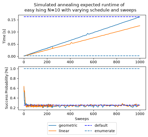
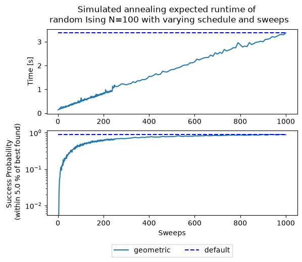
These plots represent ofter contradictory metrics, on one hand you would like to obtain a large probability of finding a right solution (the deffinition of right comes from what you define as success). On the other hand, the time it takes to solve these cases should be as small as possible. This is why we are interested in a metric that combines both, and that is why we settle on the Time To Solution (TTS) which is defined as

TTS = \frac{\log{1-s}}{\log{1-p}}

(10)

where s is a success factor, usually takes as $s = 99\%$ , and $p$ is the success probability, usually accounted as the observed success probability.

One usually reads this as the time to solution within 99% probability.

fig1 = plt.figure()
ax1 = fig1.add_subplot(111)
for schedule in schedules:
    ax1.semilogy(sweeps, results['tts'][schedule], '-', label=schedule)


# Value for the default solution
ttsDefault = results['tts']['geometric'][-1]
ax1.hlines(ttsDefault, sweeps[0], sweeps[-1], linestyle='--', label='default', colors='b')


ax1.set_ylabel('Time To Optimal Solution with ' + str(s*100) +' % chance [s]')
ax1.set_xlabel('Sweeps')
ax1.set_title('Simulated annealing expected runtime of \n' + ' example with varying schedule and sweeps')

ax2 = plt.axes([.45, .3, .4, .4])
for schedule in schedules:
    ax2.semilogy(sweeps[0:5],results['tts'][schedule][0:5],'-s')
ax2.set_ylabel('TTS [s]')
ax2.set_xlabel('Sweeps')


ax1.legend(ncol = 2, loc='upper center', bbox_to_anchor=(0.5, -0.15))

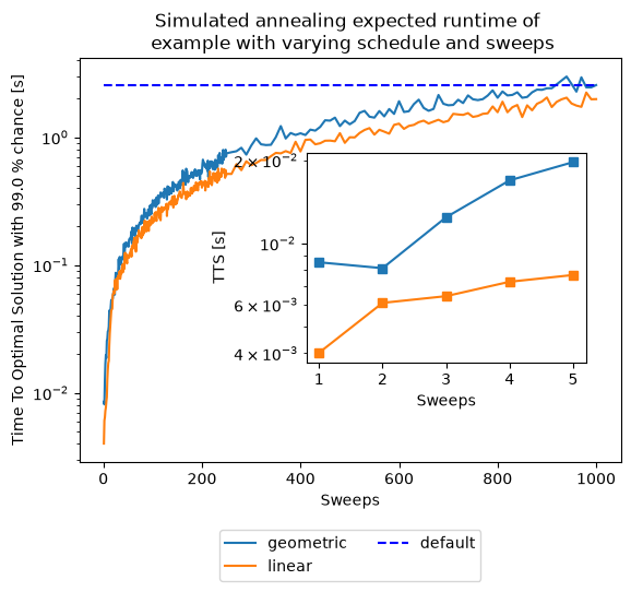
As you can notice, the default parameters given by D-Wave (number of sweeps = 1000 and a geometric update of $\beta$ ) are not optimal for our tiny example in terms of expected runtime. This is certainly a function of the problem, for such a small instance having two sweeps are more than enough and more sweeps are an overkill. This parameters choice might not generalize to any other problem, as seen below.

Random-instance benchmark¶

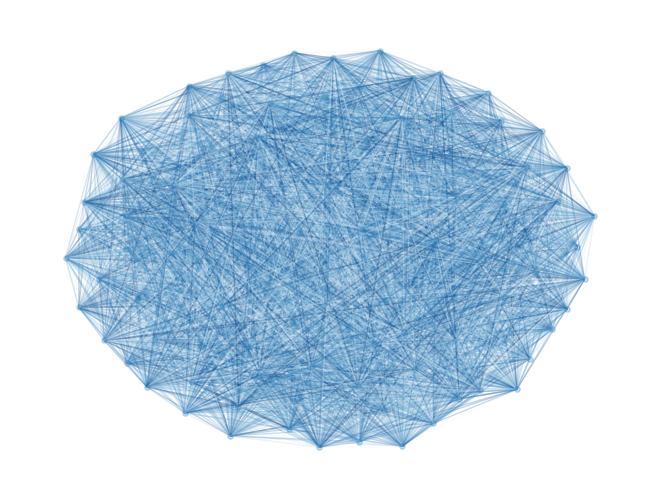
Let’s define a larger model, with 100 variables and random weights, to see how this performance changes.

Assume that we are interested in an instance with random weights $h_{i}, J_{i, j} \sim U[-1, +1]$ .

N = 100 # Number of variables
np.random.seed(42) # Fixing the random seed to get the same result
J = 2 * np.random.rand(N, N) - 1
J = np.triu(J, 1) # We only consider upper triangular matrix ignoring the diagonal
h = 2 * np.random.rand(N) - 1

model_random = dimod.BinaryQuadraticModel.from_ising(h, J, offset=0.0)

nx_graph = dimod.to_networkx_graph(model_random)
edges, bias = zip(*nx.get_edge_attributes(nx_graph, 'bias').items())
bias = np.array(bias)
nx.draw(nx_graph, node_size=15, pos=nx.spring_layout(nx_graph), alpha=0.25, edgelist=edges, edge_color=bias, edge_cmap=plt.cm.Blues)

For a problem of this size we cannot do a complete enumeration ( $2^{100} \approx 1.2e30$ ) but we can randomly sample the distribution of energies to have a baseline for our later comparisons.

randomSampler = dimod.RandomSampler()
randomSample = randomSampler.sample(model_random, seed=314159, num_reads=1000)
energies = [datum.energy for datum in randomSample.data(
        ['energy'], sorted_by='energy')]
random_energy = np.mean(energies)
print('Average random energy:' + str(random_energy))

Average random energy:0.8893359888718223

plot_energy_values(randomSample,
               title='Random sampling')

minimum energy: -114.83700225525205

<Axes: title={'center': 'Random sampling'}, xlabel='solution', ylabel='Energy'>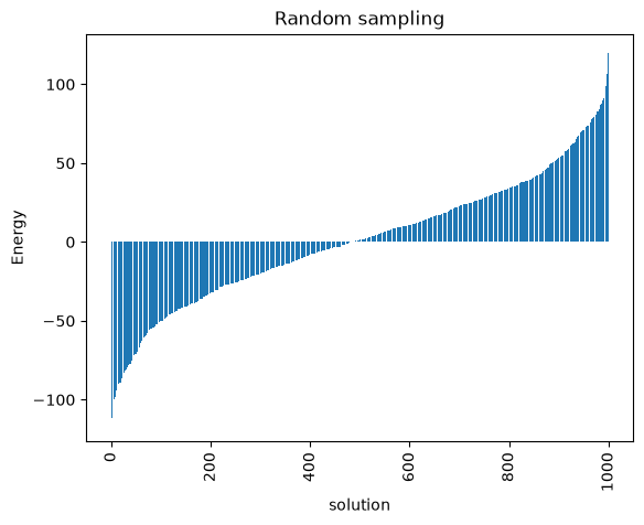

start = time.time()
simAnnSamplesDefault = simAnnSampler.sample(model_random, seed=314159, num_reads=1000)
timeDefault = time.time() - start
energies = [datum.energy for datum in simAnnSamplesDefault.data(
        ['energy'], sorted_by='energy')]
min_energy = energies[0]
print("minimum energy: " + str(min_energy))
print("runtime: " + str(timeDefault) + " seconds")

minimum energy: -424.47469301518714
runtime: 1.7792482376098633 seconds

Random-instance problem statement¶

We pose the Ising problem as the following optimization problem:

\min_{s \in \{ \pm 1 \}^n} H(s) = \min_{s \in \{ \pm 1 \}^n} \sum_{(i, j) \in E(G)} J_{i,j}s_is_j + \sum_{i \in V(G)} h_is_i + \beta

(11)

ax_enum = plot_energy_values(simAnnSamplesDefault,
               title='Simulated annealing with default parameters')
ax_enum.set(ylim=[min_energy*(0.99)**np.sign(min_energy),min_energy*(1.1)**np.sign(min_energy)])
plot_energy_cfd(simAnnSamplesDefault,
              title='Simulated annealing with default parameters', skip=10)

minimum energy: -424.47469301518714

minimum energy: -424.47469301518714

<Axes: title={'center': 'Simulated annealing with default parameters'}, xlabel='Energy', ylabel='Probabilities'>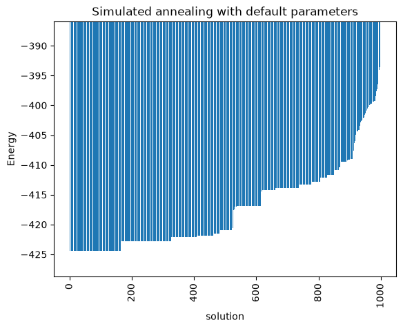

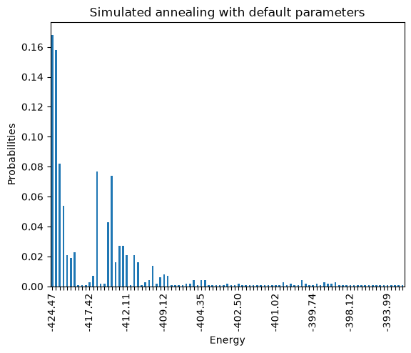
Notice that the minimum energy coming from the random sampling and the one from the simulated annealing are very different. Moreover, the distributions that both lead to are extremely different too.

print(simAnnSamplesDefault.info)
beta_schedule = np.geomspace(*simAnnSamplesDefault.info['beta_range'], num=1000)
fig, ax = plt.subplots()
ax.plot(beta_schedule,'.')
ax.set_xlabel('Sweeps')
ax.set_ylabel('beta=Inverse temperature')
ax.set_title('Default Geometric temperature schedule')

{'beta_range': [np.float64(0.006275211137529919), np.float64(32300.48293714536)], 'beta_schedule_type': 'geometric', 'timing': {'preprocessing_ns': 10681407, 'sampling_ns': 1768027756, 'postprocessing_ns': 405698}}

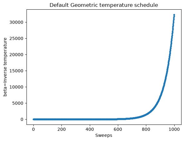
We can solve this problem using IP such that we have guarantees that it is solved to optimality (this might be a great quiz for future lectures), but in this case let us define the “success” as getting an objective certain percentage of the best found solution in all cases (which we see it might not be even found with the default parameters). To get a scaled version of this success equivalent for all instances, we will define this success with respect to the metric:

\frac{found - random}{minimum - random}

(12)

Where $found$ corresponds to the best found solution within our sampling, $random$ is the mean of the random sampling shown above, and $minimum$ corresponds to the best found solution to our problem during the exploration. Consider that this minimum might not be the global minimum. The best possible performance ratio is 1, attained at the best-known value; a negative ratio means the method performs worse than random sampling. Success is now counted as being within a specified threshold of this value of 1. We will refer to this quality of solution metric as Performance Ratio.

Before figuring out if we have the right optimal parameters, we want to save some effort by loading previously computed results. Run the next cell to download the precomputed benchmark cache before continuing. Skipping this download, or changing overwrite_pickles to regenerate the data, can trigger approximately 3 hours of local computation. Otherwise, a zip file with precomputed results will be downloaded from GitHub.

from pathlib import Path
from urllib.request import urlretrieve
import shutil

current_path = Path.cwd()
pickle_path = current_path / 'results'
pickle_path.mkdir(exist_ok=True)

zip_name = pickle_path / 'results.zip'
bundled_zip = current_path / 'results.zip'
if not zip_name.exists():
    if bundled_zip.exists():
        shutil.copyfile(bundled_zip, zip_name)
    else:
        urlretrieve(
            'https://github.com/JuliaQUBO/QUBONotebooks/raw/main/notebooks_py/results.zip',
            zip_name,
        )

pickle_path = str(pickle_path)

import zipfile
import json

zip_name = os.path.join(pickle_path, 'results.zip')
overwrite_pickles = False
if os.path.exists(zip_name):
    with zipfile.ZipFile(zip_name, 'r') as zip_ref:
        zip_ref.extractall(pickle_path)
    print('Results zip file has been extracted to ' + pickle_path)

def benchmark_cache_to_json(value):
    if isinstance(value, dict):
        return {str(key): benchmark_cache_to_json(item) for key, item in value.items()}
    if isinstance(value, (list, tuple)):
        return [benchmark_cache_to_json(item) for item in value]
    if isinstance(value, np.ndarray):
        return benchmark_cache_to_json(value.tolist())
    if isinstance(value, np.generic):
        return benchmark_cache_to_json(value.item())
    if isinstance(value, float):
        if math.isinf(value):
            return 'Infinity' if value > 0 else '-Infinity'
        if math.isnan(value):
            return 'NaN'
    return value

def benchmark_cache_from_json(value):
    if isinstance(value, dict):
        converted = {}
        for key, item in value.items():
            try:
                normalized_key = int(key)
            except (TypeError, ValueError):
                normalized_key = key
            converted[normalized_key] = benchmark_cache_from_json(item)
        return converted
    if isinstance(value, list):
        return [benchmark_cache_from_json(item) for item in value]
    if value == 'Infinity':
        return np.inf
    if value == '-Infinity':
        return -np.inf
    if value == 'NaN':
        return np.nan
    return value

def normalize_single_results_cache(results):
    if 'ttt' in results and 'tts' not in results:
        results['tts'] = results.pop('ttt')
    if 'tttci' in results and 'ttsci' not in results:
        results['ttsci'] = results.pop('tttci')
    return results

def schedule_boot_to_boot_schedule(schedule_boot):
    boot_schedule = {}
    for schedule, boot_values in schedule_boot.items():
        for boot, values in boot_values.items():
            boot_schedule.setdefault(boot, {})[schedule] = values
    return boot_schedule

def boot_schedule_to_schedule_boot(boot_schedule):
    schedule_boot = {}
    for boot, schedule_values in boot_schedule.items():
        for schedule, values in schedule_values.items():
            schedule_boot.setdefault(schedule, {})[boot] = values
    return schedule_boot

def unwrap_default_sweep(schedule_map, default_sweep_count):
    unwrapped = {}
    for schedule, values in schedule_map.items():
        if isinstance(values, dict) and default_sweep_count in values:
            unwrapped[schedule] = values[default_sweep_count]
        else:
            unwrapped[schedule] = values
    return unwrapped

def normalize_all_results_cache(all_results, default_sweep_count):
    for instance_results in all_results.values():
        normalize_single_results_cache(instance_results)
        for key in ['p', 'tts', 'ttsci', 'best', 'bestci']:
            if key in instance_results and instance_results[key]:
                first_key = next(iter(instance_results[key]))
                if isinstance(first_key, int):
                    instance_results[key] = boot_schedule_to_schedule_boot(instance_results[key])
        for key in ['t', 'min_energy', 'random_energy']:
            if key in instance_results:
                instance_results[key] = unwrap_default_sweep(instance_results[key], default_sweep_count)
    return all_results

def load_benchmark_cache(path, layout, default_sweep_count=None):
    with open(path) as file:
        data = benchmark_cache_from_json(json.load(file))
    if layout == 'single':
        return normalize_single_results_cache(data)
    if layout == 'all':
        if default_sweep_count is None:
            raise ValueError('default_sweep_count is required for all-results caches')
        return normalize_all_results_cache(data, default_sweep_count)
    raise ValueError(f'Unsupported benchmark cache layout: {layout}')

def save_benchmark_cache(path, data):
    with open(path, 'w') as file:
        json.dump(benchmark_cache_to_json(data), file, allow_nan=False)

Results zip file has been extracted to <notebook-directory>/results

Now either we have the pickled file or not, let us compute the statistics we are looking for.

success_probability = 0.99
success_threshold_percent = 5.0
benchmark_instance = 42
primary_schedule = 'geometric'
comparison_sweeps = [10, 500]
ensemble_size = 20

s = success_probability
threshold = success_threshold_percent
sweeps = list(chain(np.arange(1, 250, 1), np.arange(250, 1001, 10)))
schedules = [primary_schedule]
total_reads = 1000
default_sweeps = 1000
n_boot = 1000
ci = 68
boots = [1, 10, default_sweeps]
min_energy = -239.5
instance = benchmark_instance
results_json_name = "results_" + str(instance) + ".json"
results_json_name = os.path.join(pickle_path, results_json_name)
results_name = "results_" + str(instance) + ".pkl"
results_name = os.path.join(pickle_path, results_name)
loaded_results = None
if os.path.exists(results_json_name):
    loaded_results = load_benchmark_cache(results_json_name, layout='single')
elif os.path.exists(results_name):
    with open(results_name, "rb") as cache_file:
        loaded_results = normalize_single_results_cache(pickle.load(cache_file))
    save_benchmark_cache(results_json_name, loaded_results)
results = {}
results['p'] = {}
results['min_energy'] = {}
results['random_energy'] = {}
results['tts'] = {}
results['ttsci'] = {}
results['t']= {}
results['best'] = {}
results['bestci'] = {}
if loaded_results is not None:
    results = loaded_results
else:
    for boot in boots:
        results['p'][boot] = {}
        results['tts'][boot] = {}
        results['ttsci'][boot] = {}
        results['best'][boot] = {}
        results['bestci'][boot] = {}

    for schedule in schedules:
        probs = {k: [] for k in boots}
        time_to_sol = {k: [] for k in boots}
        prob_np = {k: [] for k in boots}
        ttscs = {k: [] for k in boots}
        times = []
        b = {k: [] for k in boots}
        bnp = {k: [] for k in boots}
        bcs = {k: [] for k in boots}
        for sweep in sweeps:
            pickle_name = str(instance) + "_" + schedule + "_" + str(sweep) + ".p"
            pickle_name = os.path.join(pickle_path, pickle_name)
            if os.path.exists(pickle_name) and not overwrite_pickles:
                with open(pickle_name, "rb") as cache_file:
                    samples = pickle.load(cache_file)
                time_s = samples.info['timing']
            else:
                start = time.time()
                samples = simAnnSampler.sample(model_random, seed=314159, num_reads=total_reads, num_sweeps=sweep, beta_schedule_type=schedule)
                time_s = time.time() - start
                samples.info['timing'] = time_s
                with open(pickle_name, "wb") as cache_file:
                    pickle.dump(samples, cache_file)
            energies=samples.data_vectors['energy']
            occurrences = samples.data_vectors['num_occurrences']
            total_counts = sum(occurrences)
            times.append(time_s)
            if min(energies) < min_energy:
                min_energy = min(energies)
                print("A better solution of " + str(min_energy) + " was found for sweep " + str(sweep))
            success = random_energy - (random_energy - min_energy)*(1.0 - threshold/100.0)
            
            boot_dist = {}
            pr_dist = {}
            cilo = {}
            ciup = {}
            pr = {}
            pr_cilo = {}
            pr_ciup = {}
            for boot in boots:
                boot_dist[boot] = []
                pr_dist[boot] = []
                for i in range(int(n_boot)):
                    resampler = np.random.randint(0, total_reads, boot)
                    sample_boot = energies.take(resampler, axis=0)
                    boot_dist[boot].append(min(sample_boot))
    
                    resampled_occurrences = occurrences.take(resampler, axis=0)
                    counts = {}
                    for index, energy in enumerate(sample_boot):
                        if energy in counts.keys():
                            counts[energy] += resampled_occurrences[index]
                        else:
                            counts[energy] = resampled_occurrences[index]
                    pr_dist[boot].append(sum(counts[key] for key in counts.keys() if key < success)/boot)   
                
                b[boot].append(np.mean(boot_dist[boot]))
                bnp[boot] = np.array(boot_dist[boot])
                cilo[boot] = np.apply_along_axis(stats.scoreatpercentile, 0, bnp[boot], 50.-ci/2.)
                ciup[boot] = np.apply_along_axis(stats.scoreatpercentile, 0, bnp[boot], 50.+ci/2.)  
                bcs[boot].append((cilo[boot],ciup[boot]))
                prob_np[boot] = np.array(pr_dist[boot])
                pr[boot] = np.mean(prob_np[boot])
                probs[boot].append(pr[boot])
                if prob_np[boot].all() == 0:
                    time_to_sol[boot].append(np.inf)
                    ttscs[boot].append((np.inf, np.inf))
                else:
                    pr_cilo[boot] = np.apply_along_axis(stats.scoreatpercentile, 0, prob_np[boot], 50.-ci/2.)
                    pr_ciup[boot] = np.apply_along_axis(stats.scoreatpercentile, 0, prob_np[boot], 50.+ci/2.)
                    time_to_sol[boot].append(time_s*math.log10(1-s)/math.log10(1-pr[boot]+1e-9)) 
                    ttscs[boot].append((time_s*math.log10(1-s)/math.log10(1-pr_cilo[boot]),time_s*math.log10(1-s)/math.log10(1-pr_ciup[boot]+1e-9)))
            
        results['t'][schedule] = times
        results['min_energy'][schedule] = min_energy
        results['random_energy'][schedule] = random_energy
        for boot in boots:
            results['p'][boot][schedule] = probs[boot]
            results['tts'][boot][schedule] = time_to_sol[boot]
            results['ttsci'][boot][schedule] = ttscs[boot]
            results['best'][boot][schedule] = [(random_energy - energy) / (random_energy - min_energy) for energy in b[boot]]
            results['bestci'][boot][schedule] = [tuple((random_energy - element) / (random_energy - min_energy) for element in energy) for energy in bcs[boot]]
    
    # Save results file in case that we are interested in reusing them
    with open(results_name, "wb") as cache_file:
        pickle.dump(results, cache_file)
    save_benchmark_cache(results_json_name, results)

schedule_for_min_sweep = primary_schedule
tts_for_min_sweep = np.asarray(results['tts'][default_sweeps][schedule_for_min_sweep], dtype=float)
min_sweep = sweeps[int(np.nanargmin(tts_for_min_sweep))]

After gathering all the results, we would like to see the progress of the Performance Ratio with respect to the increasing number of sweeps. To account for the stochasticity of this method, we are bootstrapping all of our results with different values of the bootstrapping sample, and each confidence interval corresponds to a standard deviation away from the mean.

fig, ax = plt.subplots()
for boot in boots:
    for schedule in schedules:
        ax.plot(sweeps,results['best'][boot][schedule], label=str(schedule) + ', ' + str(boot) + ' reads')
        bestnp = np.stack(results['bestci'][boot][schedule], axis=0).T
        ax.fill_between(sweeps,bestnp[0],bestnp[1],alpha=0.25)
ax.set(xlabel='Sweeps')
ax.set(ylabel='Performance Ratio = \n ' + '(best found - random sample) / (min energy - random sample)')
ax.set_title(f'Simulated annealing Performance Ratio of Ising {benchmark_instance} N=100\n' +
          ' with varying schedule, ' + str(n_boot) + ' bootstrap re-samples, and sweeps')
plt.legend(ncol=3, loc='upper center', bbox_to_anchor=(0.5, -0.15))
ax.set(xscale='log')
ax.set(ylim=[0.8,1.01])

[(0.8, 1.01)]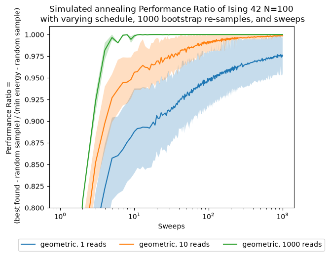

Now, besides looking at the sweeps, which are our parameter, we want to see how the performance changes with respect to the number of shots, which in this case are proportional to the computational time/effort that it takes to solve the problem.

fig, ax = plt.subplots()
for boot in boots:
    reads = [s * boot for s in sweeps]
    for schedule in schedules:
        ax.plot(reads,results['best'][boot][schedule], label=str(schedule) + ' with ' + str(boot) + ' reads')
        bestnp = np.stack(results['bestci'][boot][schedule], axis=0).T
        ax.fill_between(reads,bestnp[0],bestnp[1],alpha=0.25)
ax.set(xlabel='Total number of reads')
ax.set(ylabel='Performance Ratio = \n ' + '(best found - random sample) / (min energy - random sample)')
ax.set_title(f'Simulated annealing Performance Ratio of Ising {benchmark_instance} N=100\n' +
          ' with varying schedule, ' + str(n_boot) + ' bootstrap re-samples, and sweeps')
plt.legend(ncol=3, loc='upper center', bbox_to_anchor=(0.5, -0.15))
ax.set(xscale='log')
ax.set(ylim=[0.8,1.01])

[(0.8, 1.01)]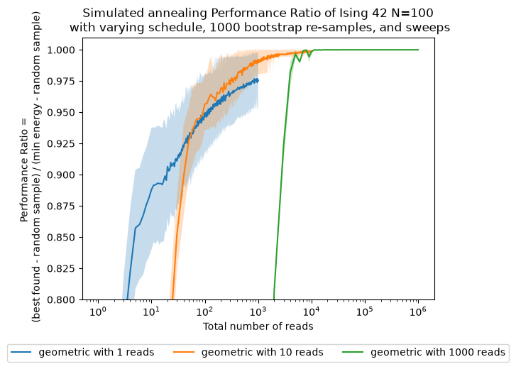

fig, (ax1,ax2) = plt.subplots(2)
fig.suptitle('Simulated annealing expected runtime of \n' +
             ' random Ising N=100 with varying schedule and sweeps')

for schedule in schedules:
    ax1.plot(sweeps, results['t'][schedule], '-', label=schedule)
ax1.hlines(results['t']['geometric'][-1], sweeps[0], sweeps[-1],
           linestyle='--', label='default', colors='b')

ax1.set(ylabel='Time [s]')
# ax1.set(xlim=[1,200])


for schedule in schedules:
    ax2.semilogy(sweeps, results['p'][default_sweeps][schedule], '-', label=schedule)
ax2.hlines(results['p'][default_sweeps]['geometric'][-1], sweeps[0], sweeps[-1],
           linestyle='--', label='default', colors='b')
# ax2.set(xlim=[1,200])

ax2.set(ylabel='Success Probability \n (within '+ str(threshold) +' % of best found)')
ax2.set(xlabel='Sweeps')
plt.legend(ncol=3, loc='upper center', bbox_to_anchor=(0.5, -0.3))

# Add plot going all the way to 1000 sweeps

import matplotlib.pyplot as plt
import numpy as np

# 1. Initialize Figure
fig1, ax1 = plt.subplots(figsize=(10, 8)) # Increased height slightly for the legend

# 2. Main Plotting Loop
for boot in reversed(boots):
    for schedule in schedules:
        ax1.plot(sweeps, results['tts'][boot][schedule], 
                 label=f"{schedule}_boot{boot}")
        ttsnp = np.stack(results['ttsci'][boot][schedule], axis=0).T
        ax1.fill_between(sweeps, ttsnp[0], ttsnp[1], alpha=0.25)

# 3. Default Horizontal Line
ax1.hlines(results['tts'][total_reads]['geometric'][-1], sweeps[0], sweeps[-1],
           linestyle='--', label='default', colors='b')

# 4. Y-Axis Settings (The Fix for 10^0)
ax1.set(yscale='log')
ax1.set(ylim=[1, 1000]) # Lower bound set to 1 (10^0)

# 5. Labels and Title
ax1.set_ylabel(f'Time To Solution within {threshold}% of best found [s]', fontsize=12)
ax1.set_xlabel('Sweeps', fontsize=12)
ax1.set_title('Simulated annealing expected runtime of random Ising N=100\n' +
             f' with varying schedule, {n_boot} bootstrap re-samples, and sweeps',
             fontsize=13, pad=20) # Increased pad for title clearance

# 6. The "No Spilling" Layout Fix
# Increase 'left' for the long y-label and 'bottom' for the external legend
plt.subplots_adjust(bottom=0.28, top=0.85, left=0.2, right=0.95) #

# 7. Legend Positioning
ax1.legend(loc='upper center', bbox_to_anchor=(0.5, -0.18),
           ncol=2, fancybox=False, shadow=False, fontsize=10)

# 8. Inset Plot (ax2)
# Adjusted coordinates to ensure it doesn't overlap the new Y-axis labels
ax2 = plt.axes([.48, .55, .38, .28]) 
for schedule in schedules:
    min_tts = min(results['tts'][default_sweeps][schedule])
    min_index = results['tts'][default_sweeps][schedule].index(min_tts)
    for boot in reversed(boots):
        ax2.semilogy(sweeps[min_index-10:min_index+10], 
                     results['tts'][boot][schedule][min_index-10:min_index+10], '-s')

ax2.set_ylabel('TTS [s]', fontsize=10)
ax2.set_xlabel('Sweeps', fontsize=10)

# 9. Final Save/Display
# Use bbox_inches='tight' to ensure the exported file captures the full text
plt.show()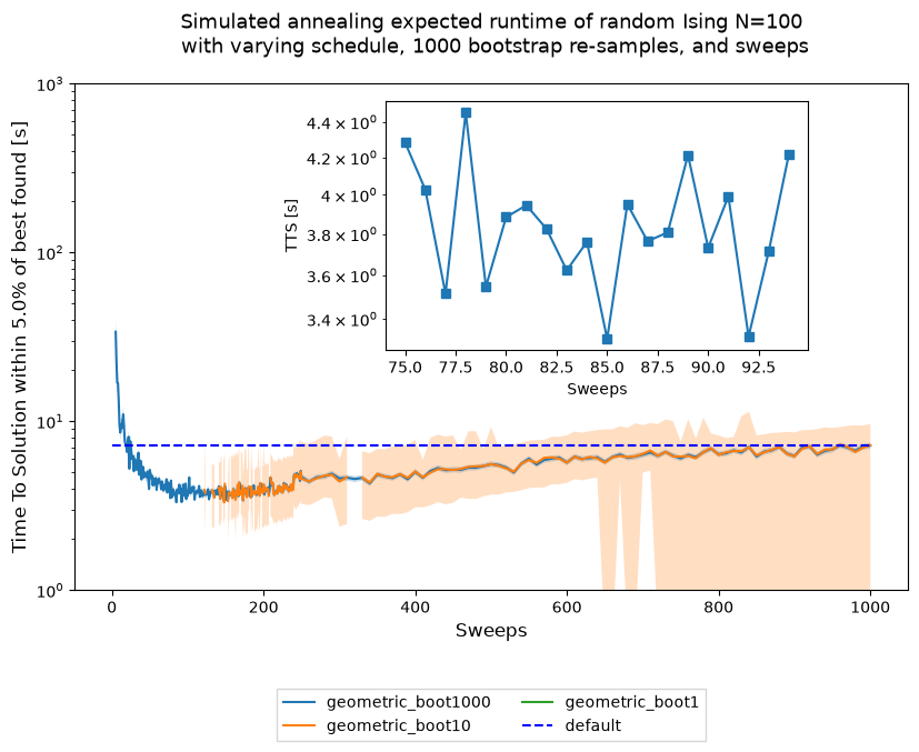

min_beta_schedule = np.geomspace(*simAnnSamplesDefault.info['beta_range'], num=min_sweep)
fig, ax = plt.subplots()
ax.plot(beta_schedule,'.')
ax.plot(min_beta_schedule,'.')
ax.set_xlabel('Sweeps')
ax.set_ylabel('beta=Inverse temperature')
ax.set_title('Geometric temperature schedule')
plt.legend(['Default','Best'])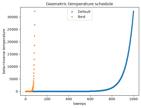

fig, ax = plt.subplots()
boots = range(1, total_reads, 1)
interest_sweeps = [min_sweep, default_sweeps, *comparison_sweeps]
approx_ratio = {}
approx_ratioci = {}

for schedule in schedules:
    approx_ratio[schedule] = {}
    approx_ratioci[schedule] = {}

instance = benchmark_instance
for sweep in interest_sweeps:
    for schedule in schedules:
        if sweep in approx_ratio[schedule] and sweep in approx_ratioci[schedule]:
            pass
        else:
            min_energy = results['min_energy'][schedule]
            random_energy = results['random_energy'][schedule]

            pickle_name = str(instance) + "_" + schedule + "_" + str(sweep) + ".p"
            pickle_name = os.path.join(pickle_path, pickle_name)
            if os.path.exists(pickle_name) and not overwrite_pickles:
                with open(pickle_name, "rb") as cache_file:
                    samples = pickle.load(cache_file)
                time_s = samples.info['timing']
            else:
                start = time.time()
                samples = simAnnSampler.sample(model_random, seed=314159, num_reads=total_reads, num_sweeps=sweep, beta_schedule_type=schedule)
                time_s = time.time() - start
                samples.info['timing'] = time_s
                with open(pickle_name, "wb") as cache_file:
                    pickle.dump(samples, cache_file)
            energies=samples.data_vectors['energy']
            if min(energies) < min_energy:
                min_energy = min(energies)
                print("A better solution of " + str(min_energy) + " was found for sweep " + str(sweep))

            b = []
            bcs = []
            probs = []
            time_to_sol = []
            for boot in boots:
                boot_dist = []
                pr_dist = []
                for i in range(int(n_boot - boot + 1)):
                    resampler = np.random.randint(0, total_reads, boot)
                    sample_boot = energies.take(resampler, axis=0)
                    boot_dist.append(min(sample_boot))   
                
                b.append(np.mean(boot_dist))
                bnp = np.array(boot_dist)
                cilo = np.apply_along_axis(stats.scoreatpercentile, 0, bnp, 50.-ci/2.)
                ciup = np.apply_along_axis(stats.scoreatpercentile, 0, bnp, 50.+ci/2.)  
                bcs.append((cilo,ciup))

            approx_ratio[schedule][sweep] = [(random_energy - energy) / (random_energy - min_energy) for energy in b]
            approx_ratioci[schedule][sweep] = [tuple((random_energy - element) / (random_energy - min_energy) for element in energy) for energy in bcs]

        ax.plot([shot*sweep for shot in boots], approx_ratio[schedule][sweep], label=str(sweep) + ' sweeps')
        approx_ratio_bestci_np = np.stack(approx_ratioci[schedule][sweep], axis=0).T
        ax.fill_between([shot*sweep for shot in boots],approx_ratio_bestci_np[0],approx_ratio_bestci_np[1],alpha=0.25)
ax.set(xscale='log')
ax.set(ylim=[0.9,1.01])
ax.set(xlim=[1e2,1e4])
ax.set(xlabel='Total number of reads (equivalent to time)')
ax.set(ylabel='Performance Ratio = \n ' + '(best found - random sample) / (min energy - random sample)')
ax.set_title(f'Simulated annealing Performance Ratio of Ising {benchmark_instance} N=100\n' +
          ' with varying schedule, ' + str(n_boot) + ' bootstrap re-samples, and sweeps')
plt.legend()

A better solution of -424.47469301518714 was found for sweep 85

A better solution of -424.47469301518714 was found for sweep 1000

A better solution of -424.47469301518714 was found for sweep 10

A better solution of -424.47469301518714 was found for sweep 500

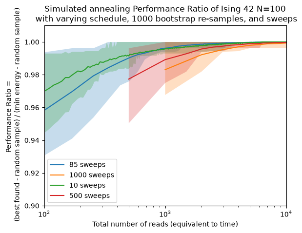
Here see how using the optimal number of sweeps is better than using other values (including the default recommended by the solver) in terms of solving this problem. Obviously, we only know this after running the experiments and verifying it ourselves. This is not the usual case, so we want to see how well can we do if we solve similar (but no the same instances). Here we will generate 20 random instances from the same distribution and size but different random seed.

Warning - long-running computation The following cell can run 20 instances x 320 sweep values x 1000 reads when the bundled cache is unavailable or overwrite_pickles is set to True. Expected runtime is about 3 hours on a standard CPU runtime.
Before running it, use the precomputed cache cells above whenever possible. If you regenerate the data, keep the browser tab open; partial JSON results are saved after each instance.


s = success_probability
threshold = success_threshold_percent
sweeps = list(chain(np.arange(1, 250, 1), np.arange(250, 1001, 10)))
schedules = [primary_schedule]
total_reads = 1000
default_sweeps = 1000
boots = [1, 10, default_sweeps]
all_results = {}
instances = range(ensemble_size)

all_results_json_name = os.path.join(pickle_path, "all_results.json")
all_results_name = "all_results.pkl"
all_results_name = os.path.join(pickle_path, all_results_name)
loaded_all_results = None
if os.path.exists(all_results_json_name):
    loaded_all_results = load_benchmark_cache(all_results_json_name, layout='all', default_sweep_count=default_sweeps)
elif os.path.exists(all_results_name):
    with open(all_results_name, "rb") as cache_file:
        loaded_all_results = normalize_all_results_cache(pickle.load(cache_file), default_sweeps)
    save_benchmark_cache(all_results_json_name, loaded_all_results)

if loaded_all_results is not None:
    all_results = loaded_all_results
else:

    for instance in tqdm(instances, desc="Instances"):
        all_results[instance] = {}
        all_results[instance]['p'] = {}
        all_results[instance]['min_energy'] = {}
        all_results[instance]['random_energy'] = {}
        all_results[instance]['tts'] = {}
        all_results[instance]['ttsci'] = {}
        all_results[instance]['t']= {}
        all_results[instance]['best'] = {}
        all_results[instance]['bestci'] = {}

        np.random.seed(instance)  # Fixing the random seed to get the same result
        J = 2 * np.random.rand(N, N) - 1
        # We only consider upper triangular matrix ignoring the diagonal
        J = np.triu(J, 1)
        h = 2 * np.random.rand(N) - 1
        model_random = dimod.BinaryQuadraticModel.from_ising(h, J, offset=0.0)

        randomSample = randomSampler.sample(model_random, seed=314159, num_reads=total_reads)
        random_energies = [datum.energy for datum in randomSample.data(
                ['energy'])]
        random_energy = np.mean(random_energies)

        default_pickle_name = str(instance) + "_" + primary_schedule + "_" + str(default_sweeps) + ".p"
        default_pickle_name = os.path.join(pickle_path, default_pickle_name)
        if os.path.exists(default_pickle_name) and not overwrite_pickles:
            with open(default_pickle_name, "rb") as cache_file:
                simAnnSamplesDefault = pickle.load(cache_file)
            timeDefault = simAnnSamplesDefault.info['timing']
        else:
            start = time.time()
            simAnnSamplesDefault = simAnnSampler.sample(model_random, seed=314159, num_reads=total_reads)
            timeDefault = time.time() - start
            simAnnSamplesDefault.info['timing'] = timeDefault
            with open(default_pickle_name, "wb") as cache_file:
                pickle.dump(simAnnSamplesDefault, cache_file)
        energies = [datum.energy for datum in simAnnSamplesDefault.data(
            ['energy'], sorted_by='energy')]
        min_energy = energies[0]
        for schedule in schedules:

            all_results[instance]['p'][schedule] = {}
            all_results[instance]['tts'][schedule] = {}
            all_results[instance]['ttsci'][schedule] = {}
            all_results[instance]['best'][schedule] = {}
            all_results[instance]['bestci'][schedule] = {}

            # probs = []
            probs = {k: [] for k in boots}
            time_to_sol = {k: [] for k in boots}
            prob_np = {k: [] for k in boots}
            ttscs = {k: [] for k in boots}
            times = []
            b = {k: [] for k in boots}
            bnp = {k: [] for k in boots}
            bcs = {k: [] for k in boots}
            for sweep in tqdm(sweeps, desc=f"Instance {instance} sweeps", leave=False):
                pickle_name = str(instance) + "_" + schedule + "_" + str(sweep) + ".p"
                pickle_name = os.path.join(pickle_path, pickle_name)
                if os.path.exists(pickle_name) and not overwrite_pickles:
                    with open(pickle_name, "rb") as cache_file:
                        samples = pickle.load(cache_file)
                    time_s = samples.info['timing']
                else:
                    start = time.time()
                    samples = simAnnSampler.sample(
                        model_random, seed=314159, num_reads=total_reads, num_sweeps=sweep, beta_schedule_type=schedule)
                    time_s = time.time() - start
                    samples.info['timing'] = time_s
                    with open(pickle_name, "wb") as cache_file:
                        pickle.dump(samples, cache_file)
                energies = samples.data_vectors['energy']
                occurrences = samples.data_vectors['num_occurrences']
                total_counts = sum(occurrences)
                times.append(time_s)
                if min(energies) < min_energy:
                    min_energy = min(energies)
                success = random_energy - (random_energy - min_energy)*(1.0 - threshold/100.0)
                
                ci = 68
                boot_dist = {}
                pr_dist = {}
                cilo = {}
                ciup = {}
                pr = {}
                pr_cilo = {}
                pr_ciup = {}
                for boot in boots:
                    boot_dist[boot] = []
                    pr_dist[boot] = []
                    for i in range(int(n_boot)):
                        resampler = np.random.randint(0, total_reads, boot)
                        sample_boot = energies.take(resampler, axis=0)
                        boot_dist[boot].append(min(sample_boot))
        
                        resampled_occurrences = occurrences.take(resampler, axis=0)
                        counts = {}
                        for index, energy in enumerate(sample_boot):
                            if energy in counts.keys():
                                counts[energy] += resampled_occurrences[index]
                            else:
                                counts[energy] = resampled_occurrences[index]
                        pr_dist[boot].append(sum(counts[key] for key in counts.keys() if key < success)/boot)
                    prob_np[boot] = np.array(pr_dist[boot])
                    pr[boot] = np.mean(prob_np[boot])
                    probs[boot].append(pr[boot])
                    
                    b[boot].append(np.mean(boot_dist[boot]))
                    bnp[boot] = np.array(boot_dist[boot])
                    cilo[boot] = np.apply_along_axis(stats.scoreatpercentile, 0, bnp[boot], 50.-ci/2.)
                    ciup[boot] = np.apply_along_axis(stats.scoreatpercentile, 0, bnp[boot], 50.+ci/2.)  
                    bcs[boot].append((cilo[boot],ciup[boot]))
                    if prob_np[boot].all() == 0:
                        time_to_sol[boot].append(np.inf)
                        ttscs[boot].append((np.inf, np.inf))
                    else:
                        pr_cilo[boot] = np.apply_along_axis(stats.scoreatpercentile, 0, prob_np[boot], 50.-ci/2.)
                        pr_ciup[boot] = np.apply_along_axis(stats.scoreatpercentile, 0, prob_np[boot], 50.+ci/2.)
                        time_to_sol[boot].append(time_s*math.log10(1-s)/math.log10(1-pr[boot]+1e-9))   
                        ttscs[boot].append((time_s*math.log10(1-s)/math.log10(1-pr_cilo[boot]+1e-9),time_s*math.log10(1-s)/math.log10(1-pr_ciup[boot]+1e-9)))
                    

            all_results[instance]['t'][schedule] = times
            all_results[instance]['min_energy'][schedule] = min_energy
            all_results[instance]['random_energy'][schedule] = random_energy
            for boot in boots:
                all_results[instance]['p'][schedule][boot] = probs[boot]
                all_results[instance]['tts'][schedule][boot] = time_to_sol[boot]
                all_results[instance]['ttsci'][schedule][boot] = ttscs[boot]
                all_results[instance]['best'][schedule][boot] = [(random_energy - energy) / (random_energy - min_energy) for energy in b[boot]]
                all_results[instance]['bestci'][schedule][boot] = [tuple((random_energy - element) / (random_energy - min_energy) for element in energy) for energy in bcs[boot]]

        save_benchmark_cache(all_results_json_name, all_results)

    # Save results file in case that we are interested in reusing them
    with open(all_results_name, "wb") as cache_file:
        pickle.dump(all_results, cache_file)
    save_benchmark_cache(all_results_json_name, all_results)

def bootstrap(data, n_boot=1000, ci=68):
    boot_dist = []
    for i in range(int(n_boot)):
        resampler = np.random.randint(0, data.shape[0], data.shape[0])
        sample = data.take(resampler, axis=0)
        # Median ignoring nans instead of mean
        boot_dist.append(np.nanmedian(sample, axis=0))
    b = np.array(boot_dist)
    s1 = np.apply_along_axis(stats.scoreatpercentile, 0, b, 50.-ci/2.)
    s2 = np.apply_along_axis(stats.scoreatpercentile, 0, b, 50.+ci/2.)
    return (s1,s2)
    
def tsplotboot(ax, x, data, error_est, **kw):
    if x is None:
        x = np.arange(data.shape[1])
    # Median ignoring nans instead of mean
    est = np.nanmedian(data, axis=0)
    mask = ~np.isnan(est)
    if error_est == 'bootstrap':
        cis = bootstrap(data)
    elif error_est == 'std':
        sd = np.nanstd(data, axis=0)
        cis = (est - sd, est + sd)
    ax.fill_between(x[mask],cis[0][mask],cis[1][mask],alpha=0.35, **kw)
    ax.plot(x[mask],est[mask],**kw)
    ax.margins(x=0)

Now we bootstrap our solutions with respect to the whole set of instances, or ensemble, and we use the median which represents the solution better than the mean.

fig, ax1 = plt.subplots()

for boot in reversed(boots):
    for schedule in schedules:
        results_array = np.array([np.array(all_results[i]['tts'][schedule][boot]) for i in instances])
        min_median_tts = min(np.nanmedian(results_array, axis=0))
        tsplotboot(ax1, x=np.asarray(sweeps), data=results_array, error_est='bootstrap', label="Ensemble " + schedule + ' with ' + str(boot) + ' reads')

        ax1.plot(sweeps,results['tts'][boot][schedule], label="Instance " + schedule + "_boot" + str(boot))


ax1.set(yscale='log')

ax1.set(ylabel='Time To Solution within '+ str(threshold) +' % of best found [s]')
ax1.set(xlabel='Sweeps')
plt.title('Simulated annealing expected runtime of \n' +
          f' Ising {benchmark_instance} N=100 with varying schedule and sweeps')

plt.legend(loc='upper center', bbox_to_anchor=(0.5, -0.2),
          ncol=3, fancybox=False, shadow=False)

ax2 = plt.axes([.45, .55, .4, .3])
inset_padding = 5
for schedule in schedules:
    results_array = np.array([np.array(all_results[i]['tts'][schedule][default_sweeps]) for i in instances])
    min_median_index = np.argmin(np.nanmedian(results_array, axis=0))
    min_median_sweep = sweeps[min_median_index]
    min_tts = min(results['tts'][default_sweeps][schedule])
    min_index = results['tts'][default_sweeps][schedule].index(min_tts)
    min_sweep = sweeps[results['tts'][default_sweeps][schedule].index(min_tts)]
    if min_sweep < min_median_sweep:
        index_lo = min_index
        index_hi = min_median_index
    else:
        index_lo = min_median_index
        index_hi = min_index
    range_lo = max(0, index_lo - inset_padding)
    range_hi = min(len(sweeps), index_hi + inset_padding)
    plot_range = slice(range_lo, range_hi)
    print("minimum median TTS for " + schedule + " schedule = " + str(min_median_tts) + "s at sweep = " + str(min_median_sweep))
    ax2.semilogy(sweeps[plot_range],
        np.median([all_results[i]['tts'][schedule][default_sweeps] for i in instances],axis=0)
        [plot_range], '-s')
    print("minimum TTS for instance " + str(benchmark_instance) + " with " + schedule + " schedule = " + str(min_tts) + "s at sweep = " + str(min_sweep))
    ax2.semilogy(sweeps[plot_range], 
        results['tts'][default_sweeps][schedule][plot_range], '-s')
    
    
ax2.hlines(np.median([all_results[i]['tts'][schedule][default_sweeps][-1] for i in instances]),
        sweeps[range_lo], sweeps[range_hi - 1],
           linestyle='--', label='default', colors='b')

ax2.set(ylabel='TTS [s]')
ax2.set(xlabel='Sweeps')

minimum median TTS for geometric schedule = infs at sweep = 112
minimum TTS for instance 42 with geometric schedule = 3.3120138340301897s at sweep = 85

[Text(0.5, 0, 'Sweeps')]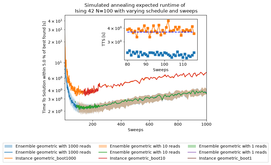

fig, ax = plt.subplots()
for boot in boots:
    for schedule in schedules:
        best_array = np.array([np.array(all_results[i]['best'][schedule][boot]) for i in instances])
        tsplotboot(ax, x=np.asarray(sweeps), data=best_array, error_est='bootstrap', label="Ensemble " + schedule + ' with ' + str(boot) + ' reads')
ax.set(xlabel='Sweeps')
ax.set(ylabel='Performance Ratio \n = best found / min energy')
ax.set_title('Simulated annealing Performance Ratio of \n' +
          ' Ensemble of Ising N=100 with varying schedule, sweeps, and number of reads')
plt.legend(ncol=3, loc='upper center', bbox_to_anchor=(0.5, -0.15))
ax.set(xscale='log')
ax.set(ylim=[0.8,1.01])

[(0.8, 1.01)]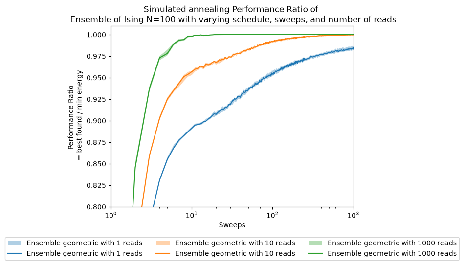

fig, ax = plt.subplots()
for boot in boots:
    reads = [s * boot for s in sweeps]
    for schedule in schedules:
        best_array = np.array([np.array(all_results[i]['best'][schedule][boot]) for i in instances])
        tsplotboot(ax, x=np.asarray(reads), data=best_array, error_est='bootstrap', label="Ensemble " + schedule + ' with ' + str(boot) + ' reads')
ax.set(xlabel='Total number of reads')
ax.set(ylabel='Performance Ratio \n = best found / min energy')
ax.set_title('Simulated annealing Performance Ratio of \n' +
          ' Ensemble of Ising N=100 with varying schedule, sweeps, and number of reads')
plt.legend(ncol=3, loc='upper center', bbox_to_anchor=(0.5, -0.15))
ax.set(xscale='log')
ax.set(ylim=[0.8,1.01])

[(0.8, 1.01)]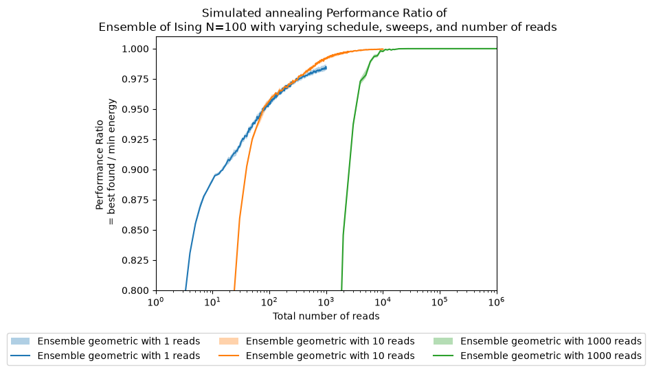

fig, ax = plt.subplots()
instance_indices = np.array(list(instances))
indices = [np.argmin(all_results[i]['tts'][primary_schedule][default_sweeps]) for i in instances]
minima = [np.min(all_results[i]['tts'][primary_schedule][default_sweeps]) for i in instances]
default = [all_results[i]['tts'][primary_schedule][default_sweeps][-1] for i in instances]
median_all = [all_results[i]['tts'][primary_schedule][default_sweeps][min_median_index] for i in instances]


ax.bar(instance_indices-0.2, minima, width=0.2, color='b', align='center', label='virtual best')
ax.bar(instance_indices, median_all, width=0.2, color='g', align='center', label='median')
ax.bar(instance_indices+0.2, default, width=0.2, color='r', align='center', label='default')
ax.xaxis.get_major_locator().set_params(integer=True)
plt.xlabel('Instance')
ax.set(ylabel='Time To Solution within '+ str(threshold) +' % of best found [s]')
plt.legend()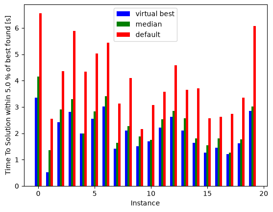

Notice how much performance would we be losing if we had used the default value for all these instances, and how much we could eventually win if we knew the best for each.

fig, ax = plt.subplots()
interest_sweeps = [min_sweep, total_reads, *comparison_sweeps]
interest_sweeps.append(min_median_sweep)
shots = range(1, total_reads, 1)
n_boot = total_reads

instance = benchmark_instance
for sweep in interest_sweeps:
    for schedule in schedules:
        if sweep in approx_ratio[schedule] and sweep in approx_ratioci[schedule]:
            pass
        else:
            min_energy = results['min_energy'][schedule]
            random_energy = results['random_energy'][schedule]
            
            pickle_name = str(instance) + "_" + schedule + "_" + str(sweep) + ".p"
            pickle_name = os.path.join(pickle_path, pickle_name)
            if os.path.exists(pickle_name) and not overwrite_pickles:
                with open(pickle_name, "rb") as cache_file:
                    samples = pickle.load(cache_file)
                time_s = samples.info['timing']
            else:
                start = time.time()
                samples = simAnnSampler.sample(model_random, seed=314159, num_reads=total_reads, num_sweeps=sweep, beta_schedule_type=schedule)
                time_s = time.time() - start
                samples.info['timing'] = time_s
                with open(pickle_name, "wb") as cache_file:
                    pickle.dump(samples, cache_file)
            energies=samples.data_vectors['energy']
            if min(energies) < min_energy:
                min_energy = min(energies)
                print("A better solution of " + str(min_energy) + " was found for sweep " + str(sweep))

            b = []
            bcs = []
            probs = []
            time_to_sol = []
            for shot in shots:
                shot_dist = []
                pr_dist = []
                for i in range(int(n_boot - shot + 1)):
                    resampler = np.random.randint(0, total_reads, shot)
                    sample_shot = energies.take(resampler, axis=0)
                    shot_dist.append(min(sample_shot))   
                
                b.append(np.mean(shot_dist))
                bnp = np.array(shot_dist)
                cilo = np.apply_along_axis(stats.scoreatpercentile, 0, bnp, 50.-ci/2.)
                ciup = np.apply_along_axis(stats.scoreatpercentile, 0, bnp, 50.+ci/2.)  
                bcs.append((cilo,ciup))
            
            approx_ratio[schedule][sweep] = [(random_energy - energy) / (random_energy - min_energy) for energy in b]
            approx_ratioci[schedule][sweep] = [tuple((random_energy - element) / (random_energy - min_energy) for element in energy) for energy in bcs]

        ax.plot([shot*sweep for shot in shots], approx_ratio[schedule][sweep], label=str(sweep) + ' sweeps')
        approx_ratio_bestci_np = np.stack(approx_ratioci[schedule][sweep], axis=0).T
        ax.fill_between([shot*sweep for shot in shots],approx_ratio_bestci_np[0],approx_ratio_bestci_np[1],alpha=0.25)
ax.set(xscale='log')
ax.set(ylim=[0.95,1.001])
ax.set(xlim=[1e2,1e4])
ax.set(xlabel='Total number of reads (equivalent to time)')
ax.set(ylabel='Performance Ratio = \n ' + '(best found - random sample) / (min energy - random sample)')
ax.set_title(f'Simulated annealing Performance Ratio of Ising {benchmark_instance} N=100\n' +
          ' with varying schedule, ' + str(n_boot) + ' bootstrap re-samples, and sweeps')
plt.legend()

A better solution of -424.47469301518714 was found for sweep 112

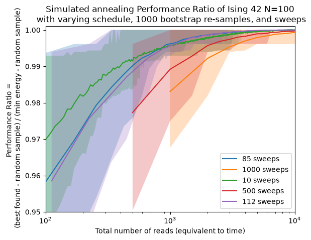
This example shows that for the benchmark instance, using the mean of the best accross the ensemble is better than using the default, but not as good as if we knew from scratch what would have made the best case.

After figuring out what would be the best parameter for our instance of interest, it would be nice to see what the ensemble performance is. We have several choices, either going with the (arbitrary) default values, or using the mean of the best performance we have found up to that point. There is an unachievable goal, which would be the case where we knew the best solution of each case, which we call the virtual best. This helps us understand how much is at stake with the choice of parameters we make.

fig, ax = plt.subplots()
default_sweeps = 1000
interest_sweeps = [min_median_sweep, default_sweeps]
interest_sweeps.append('best')
# This cell uses 100 independent bootstrap repetitions per shot count.
n_boot = 100  # Independent bootstrap repetitions for every shot count.
np.random.seed(314159)
overwrite_pickles = False


all_approx_ratio = {}

for instance in instances:
    # Rebuild this instance even when the ensemble summaries came from cache.
    # Use a local RNG so model construction does not change bootstrap draws.
    instance_rng = np.random.RandomState(instance)
    instance_J = np.triu(2 * instance_rng.rand(N, N) - 1, 1)
    instance_h = 2 * instance_rng.rand(N) - 1
    instance_model = dimod.BinaryQuadraticModel.from_ising(instance_h, instance_J)
    all_approx_ratio[instance] = {}
    for schedule in schedules:
        all_approx_ratio[instance][schedule] = {}

    for sweep in interest_sweeps:
        flag_best = False
        if sweep == 'best':
            sweep = sweeps[indices[instance]]
            flag_best = True
        for schedule in schedules:
            if sweep in all_approx_ratio[instance][schedule]:
                pass
            else:
                min_energy = all_results[instance]['min_energy'][schedule]
                random_energy = all_results[instance]['random_energy'][schedule]

                # Use a distinct cache name: older files may contain another instance.
                pickle_name = "ensemble_" + str(instance) + "_" + \
                    schedule + "_" + str(sweep) + ".p"
                pickle_name = os.path.join(pickle_path, pickle_name)
                if os.path.exists(pickle_name) and not overwrite_pickles:
                    with open(pickle_name, "rb") as cache_file:
                        samples = pickle.load(cache_file)
                    time_s = samples.info['timing']
                else:
                    start = time.time()
                    samples = simAnnSampler.sample(
                        instance_model, seed=314159, num_reads=total_reads, num_sweeps=sweep, beta_schedule_type=schedule)
                    time_s = time.time() - start
                    samples.info['timing'] = time_s
                    with open(pickle_name, "wb") as cache_file:
                        pickle.dump(samples, cache_file)
                energies = samples.data_vectors['energy']
                if min(energies) < min_energy:
                    min_energy = min(energies)

                b = []
                for shot in shots:
                    shot_dist = []
                    for i in range(n_boot):
                        resampler = np.random.randint(0, total_reads, shot)
                        sample_shot = energies.take(resampler, axis=0)
                        shot_dist.append(min(sample_shot))

                    b.append(np.mean(shot_dist))
                all_approx_ratio[instance][schedule][sweep] = [
                    (random_energy - energy) / (random_energy - min_energy) for energy in b]
            if flag_best:
                all_approx_ratio[instance][schedule]['best'] = all_approx_ratio[instance][schedule][sweep]
                ax.plot([shot*sweep for shot in shots], all_approx_ratio[instance]
                        [schedule]['best'], color='lightgray', label=None, alpha=0.5)
            else:
                ax.plot([shot*sweep for shot in shots], all_approx_ratio[instance]
                        [schedule][sweep], color='lightgray', label=None, alpha=0.25)

for sweep in interest_sweeps:
    approx_ratio_array = np.array(
        [np.array(all_approx_ratio[i][schedule][sweep]) for i in instances])
    label_plot = "Ensemble " + schedule + ' with ' + str(sweep) + ' sweeps'
    if sweep == 'best':
        sweep = sweeps[indices[instance]]
        label_plot = "Ensemble " + schedule + ' with virtual best sweeps'
    reads = [shot*sweep for shot in shots]
    tsplotboot(ax, x=np.asarray(reads), data=approx_ratio_array,
               error_est='bootstrap', label=label_plot)

ax.set(xscale='log')
ax.set(ylim=[0.95, 1.001])
ax.set(xlim=[1e2, 1e4])
ax.set(xlabel='Total number of reads (equivalent to time)')
ax.set(ylabel='Performance Ratio = \n ' +
       '(best found - random sample) / (min energy - random sample)')
ax.set_title('Simulated annealing Performance Ratio of Ising Ensemble N=100\n' +
             ' with varying schedule, ' + str(n_boot) + ' bootstrap re-samples, and sweeps')
plt.legend()

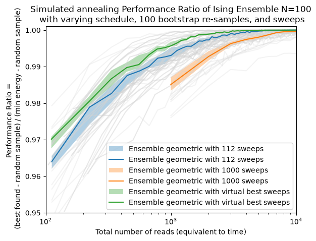
As you can see, there is a gap between the case with the best mean performance and the virtual best. This difference is arguably small, but you can imagine that with a larger number of parameters, this difference can become larger and larger, making the search of good parameters more worthy and complicated. We are actively working on such parameter setting strategies, and expect to make progress in this area (keep tuned!).

Practice checkpoints¶

Use these checkpoints during the workshop to test the main ideas before moving on.

# =============================================================================
# EXERCISE 1: Add one solver to the comparison
# =============================================================================
# Add a solver or sampler configuration to the existing benchmarking table. Record the same metrics used for the baseline solvers so the comparison is fair.
#
# Hint: Reuse the cache helpers if the run is long.
#
# Your code here:
# =============================================================================

# SOLUTION (hidden in workshop version):
# Add a new solver label to a compact benchmarking summary.
solver_results = {
    "baseline_sa": {"best_energy": -12.4, "time": 1.8},
    "new_sampler": {"best_energy": -12.6, "time": 2.1},
}
sorted_results = sorted(solver_results.items(), key=lambda item: item[1]["best_energy"])
formatted_results = [
    f"{name}: best_energy={metrics['best_energy']}, time={metrics['time']}"
    for name, metrics in sorted_results
]
print("solver_results = " + "; ".join(formatted_results))

solver_results = new_sampler: best_energy=-12.6, time=2.1; baseline_sa: best_energy=-12.4, time=1.8

# =============================================================================
# EXERCISE 2: Change the success threshold
# =============================================================================
# Compute time-to-solution using a stricter or looser solution-quality threshold. Explain how the threshold changes solver ranking.
#
# Hint: Keep the bootstrapping procedure unchanged so only the success definition changes.
#
# Your code here:
# =============================================================================

# SOLUTION (hidden in workshop version):
# Recompute time-to-solution for a changed success threshold.
import math

success_probability = 0.15
target_confidence = 0.99
reads_per_run = 100
tts_reads = math.ceil(math.log(1 - target_confidence) / math.log(1 - success_probability)) * reads_per_run
print(f"target_confidence = {target_confidence}; tts_reads = {tts_reads}")

target_confidence = 0.99; tts_reads = 2900

# =============================================================================
# EXERCISE 3: Interpret performance ratio
# =============================================================================
# Choose one instance and explain why its performance-ratio curve differs from another solver or schedule. Connect the plot shape to best, random, and observed energies.
#
# Hint: Identify where the curve is flat, steep, or noisy.
#
# Your code here:
# =============================================================================

# SOLUTION (hidden in workshop version):
# Compute a performance ratio from best, random, and observed energies.
best_energy = -15.0
random_energy = -3.0
observed_energy = -12.0
performance_ratio = (observed_energy - random_energy) / (best_energy - random_energy)
print(f"performance_ratio = {performance_ratio}")

performance_ratio = 0.75

Summary¶

In this notebook we:

Treated a solver as a combination of hardware, algorithm, software, and hyperparameters to make comparisons reproducible.
Loaded or generated benchmark samples and converted raw sampling results into success probabilities and time-to-solution metrics.
Used bootstrap summaries and performance ratios to compare schedules, sweeps, default choices, and virtual-best behavior.
Interpreted how tuning on one instance or ensemble can improve results while still leaving a gap to per-instance best choices.

Learning objectives met: You practiced setting up benchmark ensembles, computing TTS and performance ratios, using bootstrap summaries, and interpreting scaling and tuning tradeoffs.

Next steps: Proceed to Notebook 6: QCi to see another quantum-inspired solver workflow and compare its modeling interface with QUBO/BQM approaches.

Further reading:

David E. Bernal Neira — Davidson School of Chemical Engineering, Purdue University
Pedro Maciel Xavier — Davidson School of Chemical Engineering, Purdue University
Benjamin J. L. Murray — Davidson School of Chemical Engineering, Purdue University; Undergraduate Research Assistant

Acknowledgments¶

This notebook was developed by:

References¶

Rønnow, T. F., Wang, Z., Job, J., Boixo, S., Isakov, S. V., Wecker, D., Martinis, J. M., Lidar, D. A., & Troyer, M. (2014). Defining and detecting quantum speedup. Science, 345(6195), 420–424. 10.1126/science.1252319