
Setup
Google Colab
Click the badge above to open this notebook in Colab. The notebook installs or activates dependencies in the setup cells below.
Local installation
Run the following from the repository root before opening this notebook locally:
julia --project=notebooks_jl -e 'using Pkg; Pkg.instantiate()'Run the command from the repository root before opening the Julia notebook locally.
Colab Instructions
If not in a Colab notebook, continue to the next section.
Work on a copy of this notebook: File > Save a copy in Drive.
Make sure the runtime is set to Julia. If Colab opens a Python runtime, use Runtime > Change runtime type and select Julia.
Execute the following setup cell to clone the repository when needed, activate the shared notebook project, and install dependencies. The first Colab run can take several minutes.
Notebook Cell
function load_qubonotebooks_bootstrap()
    candidates = (
        joinpath(pwd(), "scripts", "notebook_bootstrap.jl"),
        joinpath(pwd(), "..", "scripts", "notebook_bootstrap.jl"),
        joinpath(pwd(), "QUBONotebooks", "scripts", "notebook_bootstrap.jl"),
        joinpath("/content", "QUBONotebooks", "scripts", "notebook_bootstrap.jl"),
    )

    for candidate in candidates
        if isfile(candidate)
            include(candidate)
            return nothing
        end
    end

    in_colab = haskey(ENV, "COLAB_RELEASE_TAG") || haskey(ENV, "COLAB_JUPYTER_IP") || isdir(joinpath("/content", "sample_data"))
    if in_colab
        repo_dir = get(ENV, "QUBONOTEBOOKS_REPO_DIR", joinpath(pwd(), "QUBONotebooks"))
        if !isdir(repo_dir)
            println("[bootstrap] Cloning JuliaQUBO/QUBONotebooks into $repo_dir")
            run(`git clone --quiet --depth 1 https://github.com/JuliaQUBO/QUBONotebooks.git $repo_dir`)
        end
        include(joinpath(repo_dir, "scripts", "notebook_bootstrap.jl"))
        return nothing
    end

    error("Could not locate scripts/notebook_bootstrap.jl from $(pwd()).")
end

load_qubonotebooks_bootstrap()

BOOTSTRAP = Base.invokelatest(QUBONotebooksBootstrap.bootstrap_notebook, "5-Benchmarking")

QUBONOTEBOOKS_REPO_DIR = BOOTSTRAP.repo_dir
JULIA_NOTEBOOKS_DIR = BOOTSTRAP.notebooks_dir
JULIA_PROJECT_DIR = BOOTSTRAP.project_dir
IN_COLAB = BOOTSTRAP.in_colab;
Activate Environment
Notebook Cell
import Pkg

python_warning_filter = "ignore:invalid escape sequence:SyntaxWarning"
python_warning_filters = String.(filter(!isempty, split(get(ENV, "PYTHONWARNINGS", ""), ",")))
if python_warning_filter ∉ python_warning_filters
    push!(python_warning_filters, python_warning_filter)
    ENV["PYTHONWARNINGS"] = join(python_warning_filters, ",")
end

if @isdefined(JULIA_PROJECT_DIR)
    Pkg.activate(JULIA_PROJECT_DIR; io = devnull)
else
    Pkg.activate(@__DIR__; io = devnull)
end
Pkg.instantiate(; io = devnull, allow_autoprecomp = false)
Learning objectives
By the end of this notebook you will be able to:
Define solver, instance, schedule, and hyperparameter ensembles for benchmarking experiments.
Compute and interpret time-to-solution, success probability, and performance-ratio summaries.
Use bootstrap summaries to compare solver settings across repeated samples and instance ensembles.
Explain the difference between default, tuned, ensemble-selected, and virtual-best parameter choices.
Prerequisites
Mathematical background: QUBO/Ising models, probability, medians, and confidence intervals.
Prior notebooks: Notebooks 2-4, especially QUBO construction and simulated/quantum annealing outputs.
Accounts required: None for the bundled cache; regenerating hardware data may require solver access.
Julia version: Julia 1.10+ with the notebook project and benchmarking dependencies instantiated.
About this notebook
A solver is the combination of hardware, algorithm, software, parameter settings, and resource limits used to solve an optimization problem. No configuration is best for every problem family or computational budget.
Tuning every parameter on the target instance consumes the same time, memory, or energy budget that the final solve is meant to conserve, and it can overfit one instance. A more realistic workflow tunes configurations offline on a representative family of training instances, then evaluates the selected configuration on held-out or previously unseen instances.
This notebook develops metrics and experiments for comparing solver configurations across repeated samples and related problem instances.
Benchmarking example
For illustration purposes, we will use an example that you are already familiar with, which is an Ising model. As a solver, we will use the DWave SA simulated annealing code.
Ising model
An Ising model represents a collection of binary spin variables with pairwise couplings and optional local fields. The objective, or energy, assigns lower values to spin configurations that better satisfy those couplings, so solving the model means finding a minimum-energy spin assignment. These models are a common benchmark for simulated annealing because the same problem family can be generated at many sizes and with different coupling distributions. We use JuMP and QUBO.jl to define Ising models and solve them with simulated annealing.
Problem statement
We pose the Ising problem as the following optimization problem:
where we optimize over spins , on a constrained graph , where the quadratic coefficients are and the linear coefficients are . We also include an arbitrary offset of the Ising model .
# QUBONOTEBOOKS_COLAB_IMPORT_CELL
Base.invokelatest(
    QUBONotebooksBootstrap.load_notebook_packages!,
    "modeling packages",
    :(begin
        using LinearAlgebra
        using JuMP
        using QUBO
    end),
);
h = [
    145.0,
    122.0,
    122.0,
    266.0,
    266.0,
    266.0,
    242.5,
    266.0,
    386.5,
    387.0,
    386.5,
]

J = [
    0  0  0 24 24 24  0 24 24 24 24
    0  0  0 24  0 24 24  0 24 24 24
    0  0  0  0 24  0 24 24 24 24 24
    0  0  0  0 24 48 24 24 48 48 48
    0  0  0  0  0 24 24 48 48 48 48
    0  0  0  0  0  0 24 24 48 48 48
    0  0  0  0  0  0  0 24 48 48 48
    0  0  0  0  0  0  0  0 48 48 48
    0  0  0  0  0  0  0  0  0 72 72
    0  0  0  0  0  0  0  0  0  0 72
    0  0  0  0  0  0  0  0  0  0  0
]

β = 1319.5

ising_model = Model()

@variable(ising_model, s_var[1:11], Spin)

@objective(ising_model, Min, s_var' * J * s_var + h' * s_var + β)

println(ising_model)
Min 24 s_var[4]*s_var[1] + 24 s_var[4]*s_var[2] + 24 s_var[5]*s_var[1] + 24 s_var[5]*s_var[3] + 24 s_var[5]*s_var[4] + 24 s_var[6]*s_var[1] + 24 s_var[6]*s_var[2] + 48 s_var[6]*s_var[4] + 24 s_var[6]*s_var[5] + 24 s_var[7]*s_var[2] + 24 s_var[7]*s_var[3] + 24 s_var[7]*s_var[4] + 24 s_var[7]*s_var[5] + 24 s_var[7]*s_var[6] + 24 s_var[8]*s_var[1] + 24 s_var[8]*s_var[3] + 24 s_var[8]*s_var[4] + 48 s_var[8]*s_var[5] + 24 s_var[8]*s_var[6] + 24 s_var[8]*s_var[7] + 24 s_var[9]*s_var[1] + 24 s_var[9]*s_var[2] + 24 s_var[9]*s_var[3] + 48 s_var[9]*s_var[4] + 48 s_var[9]*s_var[5] + 48 s_var[9]*s_var[6] + 48 s_var[9]*s_var[7] + 48 s_var[9]*s_var[8] + 24 s_var[10]*s_var[1] + 24 s_var[10]*s_var[2] + 24 s_var[10]*s_var[3] + 48 s_var[10]*s_var[4] + 48 s_var[10]*s_var[5] + 48 s_var[10]*s_var[6] + 48 s_var[10]*s_var[7] + 48 s_var[10]*s_var[8] + 72 s_var[10]*s_var[9] + 24 s_var[11]*s_var[1] + 24 s_var[11]*s_var[2] + 24 s_var[11]*s_var[3] + 48 s_var[11]*s_var[4] + 48 s_var[11]*s_var[5] + 48 s_var[11]*s_var[6] + 48 s_var[11]*s_var[7] + 48 s_var[11]*s_var[8] + 72 s_var[11]*s_var[9] + 72 s_var[11]*s_var[10] + 145 s_var[1] + 122 s_var[2] + 122 s_var[3] + 266 s_var[4] + 266 s_var[5] + 266 s_var[6] + 242.5 s_var[7] + 266 s_var[8] + 386.5 s_var[9] + 387 s_var[10] + 386.5 s_var[11] + 1319.5
Subject to
s_var[1] spin
 s_var[2] spin
 s_var[3] spin
 s_var[4] spin
 s_var[5] spin
 s_var[6] spin
 s_var[7] spin
 s_var[8] spin
 s_var[9] spin
 s_var[10] spin
 s_var[11] spin
We can visualize the graph that defines this instance using the matrix as the adjacency matrix of a graph.
# QUBONOTEBOOKS_COLAB_IMPORT_CELL
Base.invokelatest(
    QUBONotebooksBootstrap.load_notebook_packages!,
    "Plots",
    :(using Plots),
);
# Make plots look professional
Plots.default(;
    fontfamily = "Computer Modern",
    plot_titlefontsize  = 16,
    titlefontsize       = 14,
    guidefontsize       = 12,
    legendfontsize      = 10,
    tickfontsize        = 10,
)
# plot(QUBOTools.backend(ising_model))
n_nodes = size(J, 1)
θ = range(0, 2π, length = n_nodes + 1)[1:end-1] # angles for circular layout
node_x = cos.(θ)
node_y = sin.(θ)
# Create the plot
p = plot(size = (800, 800), aspect_ratio = :equal, legend = false)
# Plot edges with weights as line widths
max_weight = maximum(J)
for i in 1:n_nodes, j in (i+1):n_nodes
if J[i, j] != 0
# Edge width proportional to weight (scaled for visibility)
linewidth = 0.5 + 3 * (J[i, j] / max_weight)
# Color based on weight
color_val = J[i, j] / max_weight
edge_color = RGB(color_val, 0.2, 1 - color_val)
# Plot the edge
plot!([node_x[i], node_x[j]], [node_y[i], node_y[j]],
linewidth = linewidth, color = edge_color, alpha = 0.7)
# Add weight label at midpoint
mid_x = (node_x[i] + node_x[j]) / 2
mid_y = (node_y[i] + node_y[j]) / 2
annotate!(mid_x, mid_y, text("$(J[i,j])", 8, :black, :center))
end
end
# Plot nodes
scatter!(node_x, node_y,
markersize = 12,
markercolor = :lightblue,
markerstrokewidth = 2,
markerstrokecolor = :black,
series_annotations = text.(1:n_nodes, :black, :center, 10))
# Add node labels
for i in 1:n_nodes
annotate!(node_x[i] * 1.15, node_y[i] * 1.15, text("Node $i", 10, :blue, :center))
end
# Customize the plot
title!("Graph Representation of Coupling Matrix J")
xlabel!("")
ylabel!("")
xlims!(-1.3, 1.3)
ylims!(-1.3, 1.3)
# Display the plot
p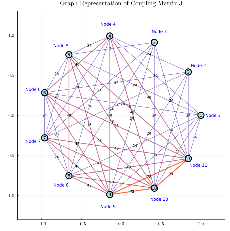
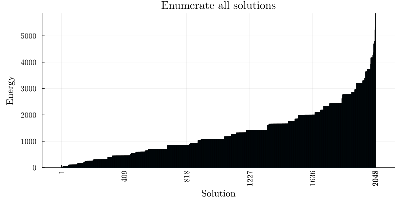
Since the problem is relatively small (11 variables, combinations), we can afford to enumerate all the solutions.
set_optimizer(ising_model, QUBO.ExactSampler.Optimizer)

optimize!(ising_model)

enumeration_time = solve_time(ising_model)

print("Enumeration took $(enumeration_time) seconds")
Enumeration took 0.414555883 seconds# Extract solution data from enumeration (immediately after optimization)
exact_solution = QUBOTools.solution(QUBOTools.backend(ising_model))
# Get all energies and occurrences
exact_energies = QUBOTools.value.(exact_solution)
exact_occurrences = QUBOTools.reads.(exact_solution)
# Sort by energy
sorted_indices = sortperm(exact_energies)
sorted_energies = exact_energies[sorted_indices]
sorted_occurrences = exact_occurrences[sorted_indices]
println("=== ENUMERATION RESULTS ===")
println("Minimum energy: ", minimum(exact_energies))
println("Total number of unique solutions: ", length(exact_energies))
println("Total number of solutions (with multiplicity): ", sum(exact_occurrences))
println("Expected: 2048 solutions for 2^11 combinations")
=== ENUMERATION RESULTS ===
Minimum energy: 5.0
Total number of unique solutions: 2048
Total number of solutions (with multiplicity): 2048
Expected: 2048 solutions for 2^11 combinations
# QUBONOTEBOOKS_COLAB_IMPORT_CELL
Base.invokelatest(
    QUBONotebooksBootstrap.load_notebook_packages!,
    "Measures",
    :(using Measures),
);
# Plot 1: Energy values for all solutions
function plot_energy_values(energies, occurrences; title=nothing)
    # Sort by energy
    sorted_indices = sortperm(energies)
    sorted_energies = energies[sorted_indices]
    sorted_occurrences = occurrences[sorted_indices]

    # Create solution indices (for x-axis)
    solution_indices = 1:length(sorted_energies)

    # Determine appropriate tick spacing for readability
    # For large datasets, show ~5 major ticks
    n_solutions = length(solution_indices)
    if n_solutions > 100
        # Calculate step size to get approximately 5 ticks
        step = max(1, div(n_solutions, 5))
        tick_positions = [1; step:step:n_solutions; n_solutions]
        tick_positions = unique(tick_positions)
        tick_labels = string.(tick_positions)
    else
        tick_positions = solution_indices
        tick_labels = string.(tick_positions)
    end

    plt = bar(solution_indices, sorted_energies,
              left_margin = 5mm,
              bottom_margin = 5mm,
              xlabel="Solution",
              ylabel="Energy",
              title=title,
              legend=false,
              size=(800, 400),
              xticks=(tick_positions, tick_labels),
              xrotation=90)  # Rotate labels vertically

    println("Minimum energy: ", minimum(energies))
    return plt
end

# Plot energy values for enumeration
plot_energy_values(exact_energies, exact_occurrences, title="Enumerate all solutions")
Minimum energy: 5.0
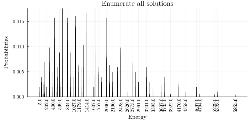
# Plot 2: Energy cumulative frequency distribution (probabilities)
function plot_energy_cfd(energies, occurrences; title=nothing, skip=1)
    # Aggregate occurrences by energy value
    energy_counts = Dict{Float64, Int}()
    for (energy, count) in zip(energies, occurrences)
        if haskey(energy_counts, energy)
            energy_counts[energy] += count
        else
            energy_counts[energy] = count
        end
    end

    # Convert to sorted arrays
    unique_energies = sort(collect(keys(energy_counts)))
    counts = [energy_counts[e] for e in unique_energies]
    total = sum(counts)
    probabilities = counts ./ total

    # Determine appropriate tick spacing for readability
    # Use energy value intervals of 200
    n_unique = length(unique_energies)
    min_energy = minimum(unique_energies)
    max_energy = maximum(unique_energies)

    if n_unique > 10
        # Create tick positions at every 200 energy interval
        # Start from the nearest multiple of 200 below min_energy, or 0 if min_energy is positive
        start_tick = max(0, floor(min_energy / 200) * 200)
        end_tick = ceil(max_energy / 200) * 200
        tick_positions = start_tick:200:end_tick

        # Find the closest actual energy values to these tick positions
        tick_energies = Float64[]
        tick_labels = String[]
        for tick_pos in tick_positions
            # Find the closest energy value
            closest_idx = argmin(abs.(unique_energies .- tick_pos))
            closest_energy = unique_energies[closest_idx]

            # Only add if it's reasonably close (within 100) or if it's the min/max
            if abs(closest_energy - tick_pos) < 100 || closest_energy == min_energy || closest_energy == max_energy
                push!(tick_energies, closest_energy)
                push!(tick_labels, string(round(closest_energy, sigdigits=7)))
            end
        end

        # Always include min and max if not already included
        if !(min_energy in tick_energies)
            tick_energies = [min_energy; tick_energies]
            tick_labels = [string(round(min_energy, sigdigits=7)); tick_labels]
        end
        if !(max_energy in tick_energies)
            push!(tick_energies, max_energy)
            push!(tick_labels, string(round(max_energy, sigdigits=7)))
        end

        # Sort to maintain order
        sort_idx = sortperm(tick_energies)
        tick_energies = tick_energies[sort_idx]
        tick_labels = tick_labels[sort_idx]
    else
        tick_energies = unique_energies
        tick_labels = [string(round(e, sigdigits=7)) for e in tick_energies]
    end

    # Create plot
    plt = bar(unique_energies, probabilities,
              left_margin = 5mm,
              bottom_margin = 10mm,
              xlabel="Energy",
              ylabel="Probabilities",
              title=title,
              legend=false,
              size=(800, 400),
              xticks=(tick_energies, tick_labels),
              xrotation=90)  # Rotate labels vertically for readability

    println("Minimum energy: ", minimum(energies))
    return plt
end

# Plot energy cumulative frequency distribution for enumeration
plot_energy_cfd(exact_energies, exact_occurrences, title="Enumerate all solutions", skip=10)
Minimum energy: 5.0
Simulated Annealing (SA)
SA is an optimization algorithm that works by navigating the input space and evaluating the objective function (energy) similarly to hill climbing. The main difference is that SA implements a strategy to avoid getting stuck in local optima.
The general idea is to allow moves to a worse position, but in a structured way. When a candidate solution is selected, the probability of actually moving to the new position is determined by the change in the objective function and by a metric called temperature. When the temperature is high, the chance of performing a jump to a worse state increases, and the opposite happens when the temperature is low. By continuously decreasing the temperature during the execution of the algorithm, it can escape local optima during the first stages (high temperature), but it settles into a position towards the end of the execution (low temperature).
Probability of Making a Jump
Case 1:
It is always advantageous to move to a state with a better objective function. In this case, the probability is .
Case 2:
In this case, the probability of taking the step is determined by:
Note: This formulation applies to a minimization problem. To solve a maximization problem, the only change is that .
Temperature Decrease
The way the temperature decreases during the algorithm’s execution varies between implementations. This is referred to as the temperature schedule, which is a function of time or the number of iterations.
Note: is also commonly used in the implementation of the algorithm.
# QUBONOTEBOOKS_COLAB_IMPORT_CELL
Base.invokelatest(
    QUBONotebooksBootstrap.load_notebook_packages!,
    "DWave",
    :(import DWave),
);
set_optimizer(ising_model, DWave.Neal.Optimizer)

set_optimizer_attribute(ising_model, "num_reads", 1_000)

optimize!(ising_model)

ising_s = round.(Int, value.(s_var))

# Display solution of the problem
println(solution_summary(ising_model))
println("* s = $ising_s")
solution_summary(; result = 1, verbose = false)
├ solver_name : D-Wave Neal Simulated Annealing Sampler
├ Termination
│ ├ termination_status : LOCALLY_SOLVED
│ ├ result_count : 12
│ └ raw_status : locally_solved
├ Solution (result = 1)
│ ├ primal_status : FEASIBLE_POINT
│ ├ dual_status : NO_SOLUTION
│ ├ objective_value      : 5.00000e+00
│ └ dual_objective_value : 1.31950e+03
└ Work counters
  └ solve_time (sec)   : 6.43423e-01
* s = [-1, -1, -1, -1, -1, -1, -1, -1, -1, -1, 1]
# Extract solution data from simulated annealing (immediately after SA optimization)
# Note: We need to get fresh solution data after the SA run
sa_solution = QUBOTools.solution(QUBOTools.backend(ising_model))

# Get all energies and occurrences
sa_energies = QUBOTools.value.(sa_solution)
sa_occurrences = QUBOTools.reads.(sa_solution)

println("=== SIMULATED ANNEALING RESULTS ===")
println("Minimum energy: ", minimum(sa_energies))
println("Total number of unique solutions: ", length(sa_energies))
println("Total number of solutions (with multiplicity): ", sum(sa_occurrences))
println("Expected: ~1000 reads from SA, but likely fewer unique solutions than enumeration")

# Verify these are different from enumeration
if length(sa_energies) == length(exact_energies) && sum(sa_occurrences) == sum(exact_occurrences)
    @warn "SA results appear identical to enumeration - this may indicate a caching issue!"
    println("Comparing first few energies:")
    println("Enumeration: ", exact_energies[1:min(5, length(exact_energies))])
    println("SA:          ", sa_energies[1:min(5, length(sa_energies))])
end
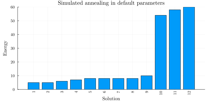
=== SIMULATED ANNEALING RESULTS ===
Minimum energy: 5.0
Total number of unique solutions: 12
Total number of solutions (with multiplicity): 1000
Expected: ~1000 reads from SA, but likely fewer unique solutions than enumeration
# Plot energy values for simulated annealing
plot_energy_values(sa_energies, sa_occurrences, title="Simulated annealing in default parameters")
Minimum energy: 5.0
# Plot energy cumulative frequency distribution for simulated annealing
plot_energy_cfd(sa_energies, sa_occurrences, title="Simulated annealing in default parameters")
Minimum energy: 5.0
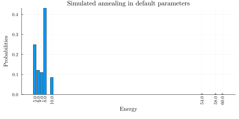
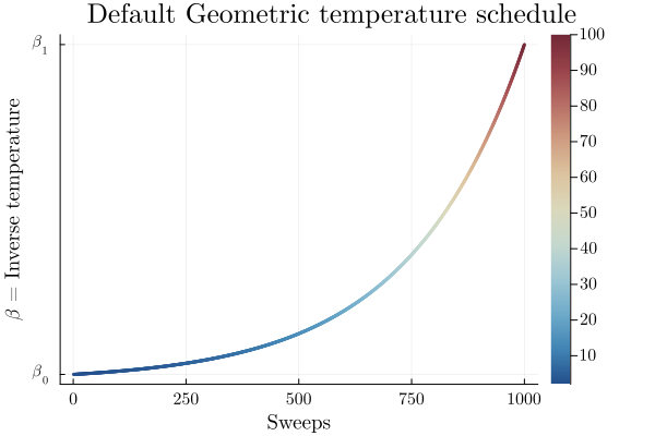
We are going to use the default limits of temperature given by the simulating annealing code. These are defined using the minimum and maximum nonzero coefficients in the Ising model. Then the range for beta is defined as
where
Hot temperature: We want to scale hot_beta so that for the most unlikely qubit flip, we get at least 50% chance of flipping. (This means all other qubits will have > 50% chance of flipping initially). Most unlikely flip is when we go from a very low energy state to a high energy state, thus we calculate hot_beta based on max_delta_energy.
Cold temperature: Towards the end of the annealing schedule, we want to minimize the chance of flipping. Don’t want to be stuck between small energy tweaks. Hence, set cold_beta so that at minimum energy change, the chance of flipping is set to 1%.
By default, the schedule also follows a geometric series.
function geomspace(a, b; length = 100)
    return exp10.(range(log10(a), log10(b); length))
end
geomspace (generic function with 1 method)# data = QUBOTools.metadata(QUBOTools.solution(qubo_model))
# info = data["info"]
β₀, β₁ = (2.0, 100.0) # info["beta_range"](2.0, 100.0)# QUBONOTEBOOKS_COLAB_IMPORT_CELL
Base.invokelatest(
QUBONotebooksBootstrap.load_notebook_packages!,
"Measures",
:(using Measures),
);
function plot_schedule(β₀, β₁; length = 1_000, title = "Default Geometric temperature schedule")
β = geomspace(β₀, β₁; length=length)
plt = plot(;
plot_title = title,
xlabel = "Sweeps",
ylabel = raw"$ \beta $ = Inverse temperature",
)
plot!(
plt, β;
right_margin = 10mm,
color = cgrad(:redblue; rev=true),
linestyle = :dot,
linewidth = 3,
line_z = β,
legend = nothing,
yticks = ([β₀, β₁], [raw"$ \beta_{0} $", raw"$ \beta_{1} $"]),
)
return plt
end
plot_schedule(β₀, β₁)
sweeps = [1:250; 260:10:1_000]
schedules = ["geometric", "linear"]
s = 0.99 # Success probability
λ⃰ = 5.0 # Optimal Energy \lambda[tab]\asteraccent[tab]
results = Dict{Symbol,Any}(
:p => Dict{String,Any}(), # Success probability
:t => Dict{String,Any}(), # Total user-observed time
:ttt => Dict{String,Any}(), # Time-to-target from total time
)
set_attribute(ising_model, "num_reads", 1_000)
for schedule in schedules
results[:p][schedule] = Float64[]
results[:t][schedule] = Float64[]
results[:ttt][schedule] = Float64[]
set_attribute(ising_model, "beta_schedule_type", schedule)
for sweep in sweeps
set_attribute(ising_model, "num_sweeps", sweep)
optimize!(ising_model)
sol = QUBOTools.solution(QUBOTools.backend(ising_model))
p = QUBOTools.success_rate(sol, λ⃰)
t = QUBOTools.total_time(sol)
ttt = QUBOTools.time_to_target(t, p, s)
push!(results[:p][schedule], p)
push!(results[:t][schedule], t)
push!(results[:ttt][schedule], ttt)
end
end
resultsDict{Symbol, Any} with 3 entries:
:p => Dict{String, Any}("geometric"=>[0.626, 0.558, 0.424, 0.394, 0.375, 0.…
:ttt => Dict{String, Any}("geometric"=>[0.0358034, 0.0481117, 0.0650856, 0.07…
:t => Dict{String, Any}("geometric"=>[0.00764632, 0.00852967, 0.00779652, 0…function plot_schedule_grid(sweeps, schedules, results)
plt = plot(;
layout = @layout([a{0.475h}; b{0.475h}; leg{0.05h}]),
size = (600, 600),
plot_title = raw"""
Simulated annealing expected total runtime of easy
$ n = 11 $ Ising model with varying schedule and sweeps
""",
plot_titlevspan = 0.1,
)
# Total user-observed time
plot!(
plt;
subplot = 1,
ylabel = "Total time [s]",
yscale = :log10,
yticks = 10.0.^(-2:1), # Explicit ticks for log scale to avoid warnings
legend = false,
)
for schedule in schedules
plot!(
plt, sweeps, results[:t][schedule];
subplot = 1,
linestyle = :solid,
label = schedule,
linewidth = 3,
)
end
hline!(
plt, [results[:t]["geometric"][end]];
subplot = 1,
linestyle = :dash,
label = "default",
color = :gray,
linewidth = 1,
)
hline!(
plt, [enumeration_time];
subplot = 1,
linestyle = :dash,
label = "enumeration",
color = :black,
linewidth = 1,
)
# Success probability
plot!(
plt;
subplot = 2,
xlabel = "Sweeps",
ylabel = "Success Probability [%]",
legend = false,
)
for schedule in schedules
plot!(
plt, sweeps, results[:p][schedule];
subplot = 2,
linestyle = :solid,
label = schedule,
ymirror = true,
linewidth = 3,
)
end
hline!(
plt, [results[:p]["geometric"][end]];
subplot = 2,
linestyle = :dash,
label = "default",
color = :gray,
linewidth = 1,
)
hline!(
plt, [1.0];
subplot = 2,
linestyle = :dash,
label = "enumeration",
color = :black,
linewidth = 1,
)
# Legend
plot!(
plt, (1:4)';
subplot = 3,
framestyle = nothing,
showaxis = false,
grid = false,
linestyle = [:solid :solid :dash :dash],
color = [1 2 :gray :black],
label = ["geometric" "linear" "default" "enumeration"],
linewidth = [3 3 1 1],
legend = :top,
legend_column = 4,
)
return plt
end
plot_schedule_grid(sweeps, schedules, results)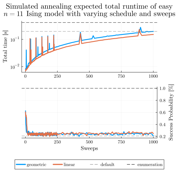
These plots represent often contradictory metrics: on one hand you would like to obtain a large probability of finding a right solution (the definition of right comes from what you define as success).
On the other hand, the time it takes to solve these cases should be as small as possible.
In this notebook, time means QUBOTools.total_time(sol): the full user-observed solution gathering time. QUBOTools.effective_time(sol) is useful for algorithm-only comparisons that exclude access, precompilation, and other overhead, but it is not the timing convention used below.
This is why we are interested in a metric that combines both, and that is why we settle on the Time To Solution (TTS) which is defined as
where is the total user-observed time, is a success factor, usually taken as , and is the success probability, usually accounted as the observed success probability.
One usually reads this as the time to solution within probability.
function plot_ttt_grid(sweeps, schedules, results, k = 20)
plt = plot(;
layout = @layout([a{0.95h}; leg{0.05h}]),
size = (700, 600),
plot_title = raw"""
Simulated annealing expected total runtime of easy
$ n = 11 $ Ising model with varying schedule and sweeps
""",
plot_titlevspan = 0.1,
plot_titlefont = Plots.font(16, "Computer Modern"),
titlefont = Plots.font(14, "Computer Modern"),
guidefont = Plots.font(12, "Computer Modern"),
legendfont = Plots.font(10, "Computer Modern"),
tickfont = Plots.font(10, "Computer Modern"),
inset_subplots = [(1, bbox(0.25,0.166,0.4,0.4, :center))],
)
# Total time-to-target
plot!(
plt;
subplot = 1,
xlabel = "Sweeps",
ylabel = "Total time to target with \$ $(100s) \\% \$ chance [s]",
legend = false,
legend_column = 3,
)
for schedule in schedules
plot!(
plt, sweeps[k+1:end], results[:ttt][schedule][k+1:end];
subplot = 1,
linestyle = :solid,
label = schedule,
yscale = :log10,
yticks = 10.0.^(-2:1), # Explicit ticks for log scale to avoid warnings
linewidth = 3,
)
end
# Value for the default solution
hline!(
plt, [results[:ttt]["geometric"][end]];
subplot = 1,
linestyle = :dash,
label = "default",
color = :gray,
linewidth = 1,
)
# Legend
plot!(
plt, (1:3)';
subplot = 2,
framestyle = nothing,
showaxis = false,
grid = false,
linestyle = [:solid :solid :dash],
linewidth = [3 3 1],
color = [1 2 :gray],
label = ["geometric" "linear" "default"],
legend = :top,
legend_column = 3,
)
plot!(
plt[3];
xlabel = "Sweeps",
ylabel = "Total TTT [s]",
yscale = :log10,
yticks = 10.0.^(-2:1), # Explicit ticks for log scale to avoid warnings
legend = false,
framestyle = :box,
)
for schedule in schedules
plot!(
plt[3], sweeps[1:k], results[:ttt][schedule][1:k];
linewidth = 2,
marker = :diamond,
markersize = 4,
)
end
hline!(
plt[3], [results[:ttt]["geometric"][end]];
linestyle = :dash,
color = :gray,
linewidth = 1,
)
return plt
end
plot_ttt_grid(sweeps, schedules, results)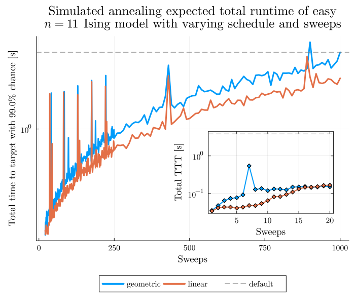
As you can notice, the default parameters given by D-Wave (number of sweeps = 1000 and a geometric update of ) are not optimal for our tiny example in terms of expected total runtime. This is certainly a function of the problem, for such a small instance having two sweeps are more than enough and more sweeps are an overkill. This parameters choice might not generalize to any other problem, as seen below.
Benchmarking example 2
Let’s define a larger model, with 100 variables and random weights, to see how this performance changes.
Assume that we are interested in an instance with random weights .
# QUBONOTEBOOKS_COLAB_IMPORT_CELL
Base.invokelatest(
QUBONotebooksBootstrap.load_notebook_packages!,
"Random",
:(using Random),
);
# Number of variables
n = 100
# Fixing the random seed to get the same result
Random.seed!(1)
# We only consider upper triangular matrix ignoring the diagonal
J = triu!(2rand(Float64, n, n) .- 1, 1)
h = 2rand(Float64, n) .- 1
;plot(QUBOTools.SystemLayoutPlot((J + J') / 2 + diagm(h)))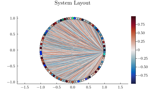
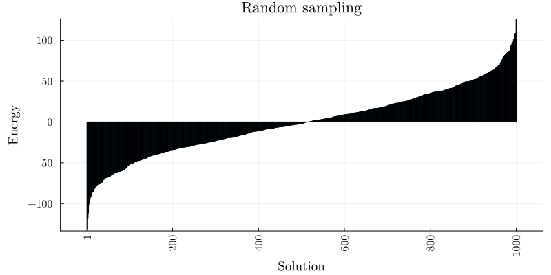
For a problem of this size we cannot do a complete enumeration () but we can randomly sample the distribution of energies to have a baseline for our later comparisons.
random_ising_model = Model()
@variable(random_ising_model, s[1:n], Spin)
@objective(random_ising_model, Min, s' * J * s + h' * s)
random_ising_modelA JuMP Model
├ solver: none
├ objective_sense: MIN_SENSE
│ └ objective_function_type: QuadExpr
├ num_variables: 100
├ num_constraints: 100
│ └ VariableRef in QUBOTools_MOI.Spin: 100
└ Names registered in the model
└ :s# QUBONOTEBOOKS_COLAB_IMPORT_CELL
Base.invokelatest(
QUBONotebooksBootstrap.load_notebook_packages!,
"Statistics",
:(using Statistics),
);
set_optimizer(random_ising_model, QUBO.RandomSampler.Optimizer)
set_attribute(random_ising_model, "num_reads", 1_000)
optimize!(random_ising_model)
random_sampling_time = solve_time(random_ising_model)
energies = [objective_value(random_ising_model; result = i) for i = 1:result_count(random_ising_model)]
random_mean_energy = mean(energies)
println("Average random energy = $(random_mean_energy)")Average random energy = -0.7062486495361374
# Extract solution data from random sampling
random_solution = QUBOTools.solution(QUBOTools.backend(random_ising_model))
# Get all energies and occurrences
random_energies = QUBOTools.value.(random_solution)
random_occurrences = QUBOTools.reads.(random_solution)
# Plot energy values for random sampling
plot_energy_values(random_energies, random_occurrences, title="Random sampling")
Minimum energy: -133.4415555415882
set_optimizer(random_ising_model, DWave.Neal.Optimizer)
set_attribute(random_ising_model, "num_reads", 1_000)
optimize!(random_ising_model)
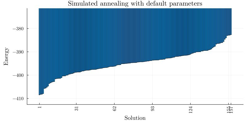
println("Simulated Annealing best energy = $(objective_value(random_ising_model))")Simulated Annealing best energy = -408.47197451530656
# Extract solution data from simulated annealing
sa_solution_default = QUBOTools.solution(QUBOTools.backend(random_ising_model))
# Get all energies and occurrences
sa_energies_default = QUBOTools.value.(sa_solution_default)
sa_occurrences_default = QUBOTools.reads.(sa_solution_default)
# Get minimum energy for ylim adjustment
min_energy_sa = minimum(sa_energies_default)
# Plot energy values for simulated annealing with ylim adjustment
plt_enum = plot_energy_values(sa_energies_default, sa_occurrences_default,
title="Simulated annealing with default parameters")
ylim_inner_scale = 0.99
ylim_outer_scale = 1.1
if min_energy_sa < 0
ylim_low = min_energy_sa / ylim_inner_scale
ylim_high = min_energy_sa / ylim_outer_scale
else
ylim_low = min_energy_sa * ylim_inner_scale
ylim_high = min_energy_sa * ylim_outer_scale
end
plot!(plt_enum, ylims=(ylim_low, ylim_high))
plt_enum
Minimum energy: -408.47197451530656
# Plot energy cumulative frequency distribution for simulated annealing
plot_energy_cfd(sa_energies_default, sa_occurrences_default,
title="Simulated annealing with default parameters", skip=10)
Minimum energy: -408.47197451530656
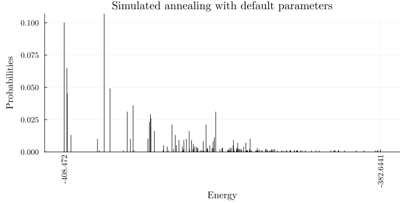
Notice that the minimum energy coming from the random sampling and the one from the simulated annealing are very different. Moreover, the distributions that both lead to are extremely different too.
# data = QUBOTools.metadata(QUBOTools.solution(qubo_model))
# info = data["info"]

β₀, β₁ = (2.0, 100.0) # info["beta_range"]
plot_schedule(β₀, β₁)We can solve this problem using IP such that we have guarantees that it is solved to optimality (this might be a great quiz for future lectures), but in this case let us define the “success” as getting an objective certain percentage of the best found solution in all cases (which we see it might not be even found with the default parameters). To get a scaled version of this success equivalent for all instances, we will define this success with respect to the metric:
Where corresponds to the best found solution within our sampling, is the mean of the random sampling shown above, and corresponds to the best found solution to our problem during the exploration. Consider that this minimum might not be the global minimum. The best possible performance ratio is 1, attained at the best-known value; a negative ratio means the method performs worse than random sampling. Success is now counted as being within a specified threshold of this value of 1. We will refer to this quality of solution metric as Performance Ratio.
Before figuring out if we have the right optimal parameters, we want to save some effort by loading previously computed results.
If you do not want to load the results that we are providing, feel free to change the overwrite_pickles variable, at the expense that it will take some time (around 3 minutes per instance) to run.
If you do not want to wait, drop the results.zip file in the folder that is about to be created.
pickle_path = joinpath(@__DIR__, "results")

if !isdir(pickle_path)
    @warn "Results directory '$pickle_path' does not exist. We will create it."

    mkpath(pickle_path)
end
┌ Warning: Results directory '<notebook-directory>/results' does not exist. We will create it.
└ @ Main In[36]:4
"<notebook-directory>/results"Put the file in there and we will decompress it for you.
# QUBONOTEBOOKS_COLAB_IMPORT_CELL
Base.invokelatest(
    QUBONotebooksBootstrap.load_notebook_packages!,
    "ZipFile",
    :(import ZipFile),
);
zip_name = joinpath(pickle_path, "results.zip")
bundled_zip = joinpath(@__DIR__, "results.zip")

if !isfile(zip_name) && isfile(bundled_zip)
    cp(bundled_zip, zip_name; force = true)
end

overwrite_pickles = false
use_raw_data = false
extract_results_archive = isfile(zip_name)

if extract_results_archive
    destination = abspath(pickle_path)
    zr = ZipFile.Reader(zip_name)

    try
        for f in zr.files
            file_path = normpath(joinpath(destination, f.name))
            relative_path = relpath(file_path, destination)

            if relative_path == ".." || startswith(relative_path, "../") || startswith(relative_path, "..\\")
                error("Refusing to extract '$(f.name)' outside '$destination'")
            end

            if endswith(f.name, "/")
                mkpath(file_path)
            else
                mkpath(dirname(file_path))
                write(file_path, read(f))
            end
        end
    finally
        close(zr)
    end

    @info("Results zip file has been extracted to '$pickle_path'")
end
[ Info: Results zip file has been extracted to '<notebook-directory>/results'
function QUBOTools.write_solution(
        io::IO,
        sol::S,
        fmt::QUBOTools.Format{:bqpjson},
        ) where {S}
    if !isempty(sol)
        metadata = QUBOTools.metadata(sol)

        json_data = Dict{String,Any}(
            "id"              => 0,
            "variable_domain" => QUBOTools._BQPJSON_VARIABLE_DOMAIN(QUBOTools.domain(sol)),
            "linear_terms"    => Dict{String,Any}[],
            "quadratic_terms" => Dict{String,Any}[],
            "variable_ids"    => 1:QUBOTools.dimension(sol),
            "scale"           => 1,
            "offset"          => 0,
            "metadata"        => metadata,
            "version"         => string(fmt[:version]),
        )

        sol_id = 0
        solutions = Dict{String,Any}[]

        for s in sol
            assignment = Dict{String,Any}[
                Dict{String,Any}("id" => i, "value" => QUBOTools.state(s, i))
                for i in 1:QUBOTools.dimension(sol)
            ]

            evaluation = QUBOTools.value(s)

            for _ = 1:QUBOTools.reads(s)
                push!(
                    solutions,
                    Dict{String,Any}(
                        "id"         => (sol_id += 1),
                        "assignment" => assignment,
                        "evaluation" => evaluation,
                    ),
                )
            end
        end

        json_data["solutions"] = solutions
        QUBOTools.JSON.print(io, json_data)
    end

    return nothing
end
function QUBOTools.read_solution(io::IO, ::QUBOTools.Format{:bqpjson})
    data = JSON.parse(io)
    grouped_solutions = Dict{Vector{Int}, Tuple{Float64, Int}}()

    for solution_data in data["solutions"]
        assignment = solution_data["assignment"]
        sort!(assignment, by = variable_value -> variable_value["id"])
        state = [Int(variable_value["value"]) for variable_value in assignment]
        energy = solution_data["evaluation"]

        if haskey(grouped_solutions, state)
            _, reads = grouped_solutions[state]
            grouped_solutions[state] = (energy, reads + 1)
        else
            grouped_solutions[state] = (energy, 1)
        end
    end

    samples = QUBOTools.Sample{Float64, Int}[]
    for (state, (energy, reads)) in grouped_solutions
        push!(samples, QUBOTools.Sample{Float64, Int}(state, energy, reads))
    end
    sort!(samples, by = QUBOTools.value)

    metadata = Dict{String, Any}(string(k) => v for (k, v) in get(data, "metadata", Dict()))
    return QUBOTools.SampleSet{Float64, Int}(
        samples;
        metadata = metadata,
        sense = :min,
        domain = :spin,
    )
end
Now either we have the pickled file or not, let us compute the statistics we are looking for.
# QUBONOTEBOOKS_COLAB_IMPORT_CELL
Base.invokelatest(
    QUBONotebooksBootstrap.load_notebook_packages!,
    "analysis packages",
    :(begin
        using Statistics
        using JSON
        using StatsBase
    end),
);
success_probability = 0.99
success_threshold_percent = 5.0
benchmark_instance = 42
primary_schedule = "geometric"
comparison_sweeps = [10, 500]
ensemble_instance_count = 20
ensemble_instances = 0:(ensemble_instance_count - 1)

s         = success_probability
threshold = success_threshold_percent

sweeps    = [1:250;260:10:1_000]
schedules = ["geometric", "linear"]

total_reads    = 1_000
default_sweeps = 1_000
n_boot         = 500
ci             = 68  # Confidence interval for bootstrapping
default_boots  = default_sweeps

boots = [1, 10, default_boots]

min_energy = -239.7094652034834
random_energy = random_mean_energy

instance     = benchmark_instance
results_name = "results_$(instance).json"
results_name = joinpath(pickle_path, results_name)
results = Dict{Symbol,Any}(
    :p             => Dict{Int,Any}(),
    :min_energy    => Dict{String,Any}(),
    :random_energy => Dict{String,Any}(),
    :ttt           => Dict{Int,Any}(),
    :tttci         => Dict{Int,Any}(),
    :t             => Dict{String,Any}(),
    :best          => Dict{Int,Any}(),
    :bestci        => Dict{Int,Any}(),
)

function benchmark_cache_to_json(value)
    if value isa AbstractDict
        return Dict{String, Any}(string(k) => benchmark_cache_to_json(v) for (k, v) in value)
    elseif value isa Tuple || value isa AbstractVector
        return [benchmark_cache_to_json(v) for v in value]
    elseif value isa Number && !isfinite(value)
        if isnan(value)
            return "NaN"
        elseif value > 0
            return "Infinity"
        else
            return "-Infinity"
        end
    end
    return value
end

function benchmark_cache_from_json(value)
    if value isa AbstractDict
        return Dict{String, Any}(string(k) => benchmark_cache_from_json(v) for (k, v) in value)
    elseif value isa AbstractVector
        return [benchmark_cache_from_json(v) for v in value]
    elseif value == "Infinity"
        return Inf
    elseif value == "-Infinity"
        return -Inf
    elseif value == "NaN"
        return NaN
    end
    return value
end

function export_summary_results(raw)
    return Dict{String, Any}(
        "p"             => benchmark_cache_to_json(raw[:p]),
        "min_energy"    => benchmark_cache_to_json(raw[:min_energy]),
        "random_energy" => benchmark_cache_to_json(raw[:random_energy]),
        "tts"           => benchmark_cache_to_json(raw[:ttt]),
        "ttsci"         => benchmark_cache_to_json(raw[:tttci]),
        "t"             => benchmark_cache_to_json(raw[:t]),
        "best"          => benchmark_cache_to_json(raw[:best]),
        "bestci"        => benchmark_cache_to_json(raw[:bestci]),
    )
end

if use_raw_data || !isfile(results_name)
    overwrite_pickles = false

    for boot in boots
        results[:p][boot]      = Dict()
        results[:ttt][boot]    = Dict()
        results[:tttci][boot]  = Dict()
        results[:best][boot]   = Dict()
        results[:bestci][boot] = Dict()
    end

    for schedule in schedules
        probs       = Dict{Int,Any}(k => [] for k in boots)
        time_to_sol = Dict{Int,Any}(k => [] for k in boots)
        prob_np     = Dict{Int,Any}(k => [] for k in boots)
        tttcs       = Dict{Int,Any}(k => [] for k in boots)
        times       = []
        b           = Dict{Int,Any}(k => [] for k in boots)
        bnp         = Dict{Int,Any}(k => [] for k in boots)
        bcs         = Dict{Int,Any}(k => [] for k in boots)

        for sweep in sweeps
            # Single-instance cache: the key includes total_reads because this sweep study reuses one benchmark instance.
            solution_name = joinpath(pickle_path, "solutions_$(total_reads)_$(sweep)_$(schedule).json")

            if isfile(solution_name) && !overwrite_pickles
                sol    = QUBOTools.read_solution(solution_name)
                time_s = QUBOTools.total_time(sol)
            else
                set_attribute(random_ising_model, "num_reads", total_reads)
                set_attribute(random_ising_model, "num_sweeps", sweep)
                set_attribute(random_ising_model, "beta_schedule_type", schedule)

                optimize!(random_ising_model)

                sol = QUBOTools.solution(QUBOTools.backend(random_ising_model))
                time_s = QUBOTools.total_time(sol)

                open(solution_name, "w") do io
                    QUBOTools.write_solution(io, sol, QUBOTools.Format{:bqpjson}())
                end
            end

            energies     = QUBOTools.value.(sol)
            occurrences  = QUBOTools.reads.(sol)
            total_counts = sum(occurrences)

            push!(times, time_s)

            if minimum(energies) < min_energy
                min_energy = minimum(energies)
                @info("A better solution of '$(min_energy)' was found for sweep '$sweep'")
            end

            success = random_energy - (random_energy - min_energy)*(1.0 - threshold/100.0)

            boot_dist = Dict{Int,Any}()
            pr_dist   = Dict{Int,Any}()
            cilo = Dict{Int,Any}()
            ciup = Dict{Int,Any}()
            pr = Dict{Int,Any}()
            pr_cilo = Dict{Int,Any}()
            pr_ciup = Dict{Int,Any}()

            for boot in boots
                boot_dist[boot] = []
                pr_dist[boot]   = []

                for i in 1:n_boot
                    resampler = rand(1:min(total_reads, length(energies)), boot)
                    sample_boot = energies[resampler]

                    push!(boot_dist[boot], minimum(sample_boot))

                    resampled_occurrences = occurrences[resampler]
                    counts     = Dict{Float64,Int}()

                    for (index, energy) in enumerate(sample_boot)
                        if energy in keys(counts)
                            counts[energy] += resampled_occurrences[index]
                        else
                            counts[energy] = resampled_occurrences[index]
                        end
                    end

                    try
                        push!(
                            pr_dist[boot],
                            sum(counts[key] for key in keys(counts) if key < success) / boot
                        )
                    catch e
                        push!(
                            pr_dist[boot],
                            0
                        )
                    end
                end

                push!(b[boot], mean(boot_dist[boot]))

                bnp[boot]  = boot_dist[boot]
                cilo[boot] = percentile(bnp[boot], 50 - ci / 2)
                ciup[boot] = percentile(bnp[boot], 50 + ci / 2)

                push!(bcs[boot], (cilo[boot], ciup[boot]))

                prob_np[boot] = pr_dist[boot]
                pr[boot]      = mean(prob_np[boot])
                if pr[boot] >= 1
                    pr[boot] = 1 - 1E-9
                end

                push!(probs[boot], pr[boot])

                if !all(x -> x > 0, prob_np[boot])
                    push!(time_to_sol[boot], Inf)
                    push!(tttcs[boot], (Inf, Inf))
                else

                    pr_cilo[boot] = percentile(prob_np[boot], 50 - ci / 2)
                    if pr_cilo[boot] >= 1
                        pr_cilo[boot] = 1 - 1E-9
                    end

                    pr_ciup[boot] = percentile(prob_np[boot], 50 + ci / 2)
                    if pr_ciup[boot] >= 1
                        pr_ciup[boot] = 1 - 1E-9
                    end

                    try
                        push!(time_to_sol[boot], time_s * log10(1-s) / log10(1 - pr[boot] + 1E-9))
                        push!(
                            tttcs[boot],
                            (
                                time_s*log10(1-s)/log10(1 - pr_cilo[boot]),
                                time_s*log10(1-s)/log10(1 - pr_ciup[boot])
                            )
                        )
                    catch e
                        println(s)
                        println(pr[boot] + 1E-9)
                        println(pr_cilo[boot])
                        println(pr_ciup[boot])
                        println(1-pr_ciup[boot])
                        throw(e)
                    end
                end
            end
        end

        results[:t][schedule]             = times
        results[:min_energy][schedule]    = min_energy
        results[:random_energy][schedule] = random_energy

        for boot in boots
            results[:p][boot][schedule]     = probs[boot]
            results[:ttt][boot][schedule]   = time_to_sol[boot]
            results[:tttci][boot][schedule] = tttcs[boot]
            results[:best][boot][schedule]  = [
                (random_energy - energy) / (random_energy - min_energy)
                for energy in b[boot]
            ]
            results[:bestci][boot][schedule] = [
                tuple(((random_energy - element) / (random_energy - min_energy) for element in energy)...)
                for energy in bcs[boot]
            ]
        end
    end

    open(results_name, "w") do io
        JSON.print(io, export_summary_results(results))
    end
else  # Just reload processed datafile
    string_dict = JSON.parsefile(results_name)

    key_aliases = Dict("tts" => "ttt", "ttsci" => "tttci")
    int_nested_keys = Set([:p, :ttt, :tttci, :best, :bestci])
    results = Dict{Symbol, Any}()

    for (k_str, v) in string_dict
        k_sym = Symbol(get(key_aliases, k_str, k_str)) # Convert top-level key to Symbol

        if k_sym in int_nested_keys
            results[k_sym] = Dict(parse(Int, sub_k) => benchmark_cache_from_json(sub_v) for (sub_k, sub_v) in v)
        else
            results[k_sym] = benchmark_cache_from_json(v)
        end
    end
end

println("Loaded benchmark results for instance $(benchmark_instance) with schedules: $(sort(collect(keys(results[:t]))))")
After gathering all the results, we would like to see the progress of the Performance Ratio with respect to the increasing number of sweeps. To account for the stochasticity of this method, we are bootstrapping all of our results with different values of the bootstrapping sample, and each confidence interval corresponds to a standard deviation away from the mean.
function plot_progress(sweeps, boots, schedules, results)
    plt = plot(;
        plot_title = """
            Simulated annealing Performance Ratio of Ising 42 N=100
            with varying schedule, $(n_boot) bootstrap re-samples, and sweeps
            """,
        xscale     = :log10,
        xticks     = 10.0.^(0:3),  # Explicit ticks for log scale to avoid warnings
        # xlims      = (1, 200),
        ylims      = (0.8, 1.01),
        xlabel     = "Sweeps",
        ylabel     = raw"Performance Ratio = \
            $\frac{\textrm{best found} - \textrm{random sample}}\
            {\textrm{min energy} - \textrm{random sample}}$",
        legend     = :outertop,
    )


    for boot in boots
        for schedule in schedules
            bestnp = transpose(stack(results[:bestci][boot][schedule], dims=1))

            plot!(
                plt,
                sweeps, bestnp[1, :];
                fillrange = bestnp[2, :],
                fillalpha = 0.25,
            )

            plot!(
                plt,
                sweeps, results[:best][boot][schedule];
                label = "$schedule, $boot reads",
            )
        end
    end
end
Now, besides looking at the sweeps, which are our parameter, we want to see how the performance changes with respect to the number of shots, which in this case are proportional to the computational time/effort that it takes to solve the problem.
title_str = "Simulated annealing Performance Ratio of Ising $(benchmark_instance) N=100\n with varying schedule, $n_boot bootstrap re-samples, and sweeps"
ylabel_str = "Performance Ratio = \n (best found - random sample) / (min energy - random sample)"
xlabel_str = "Total number of reads"

p = plot()

schedules_to_plot = [primary_schedule]

for boot in boots
    reads = [s * boot for s in sweeps]
    for schedule in schedules_to_plot
        label_str = "$schedule with $boot reads"

        mean_line = results[:best][boot][schedule]
        ci_data = results[:bestci][boot][schedule]
        low_bound = getindex.(ci_data, 1)
        high_bound = getindex.(ci_data, 2)

        plot!(p, reads, mean_line,
              ribbon=(mean_line .- low_bound, high_bound .- mean_line),
              fillalpha=0.25,
              label=label_str)
    end
end

plot!(p,
    size = (700, 700),
    plot_titlevspan = 0.1,

    plot_title = title_str,
    xlabel = xlabel_str,
    ylabel = ylabel_str,

    xscale = :log10,
    xticks = 10.0.^(2:5),
    ylims = (0.8, 1.01),

    legend = :outerbottom,
    legend_columns = 3,

    plot_titlefont  = Plots.font(14, "Computer Modern"),
    guidefont       = Plots.font(10, "Computer Modern"),
    legendfont      = Plots.font(8, "Computer Modern"),
    tickfont        = Plots.font(10, "Computer Modern")
)

# 5. Display the final plot
display(p)
# QUBONOTEBOOKS_COLAB_IMPORT_CELL
Base.invokelatest(
QUBONotebooksBootstrap.load_notebook_packages!,
"Plots",
:(using Plots),
);
# 1. Create the two plot objects (ax1 and ax2)
p1 = plot()
schedules_to_plot = [primary_schedule]
# ax2.semilogy(...) is handled by setting yscale=:log10
p2 = plot(yscale=:log10, yticks=10.0.^(-3:1))  # Explicit ticks for log scale to avoid warnings

title_str = "Simulated annealing expected total runtime of \n instance $(benchmark_instance) Ising N=100 with varying schedule and sweeps"

for schedule in schedules_to_plot
    plot!(p1, sweeps, results[:t][schedule], label=schedule)
end

y_val_1 = results[:t][primary_schedule][end]
hline!(p1, [y_val_1], linestyle=:dash, label="default", color=:blue)

ylabel!(p1, "Total time [s]")


for schedule in schedules_to_plot
    plot!(p2, sweeps, results[:p][default_sweeps][schedule], label=schedule)
end

y_val_2 = results[:p][default_sweeps][primary_schedule][end]
hline!(p2, [y_val_2], linestyle=:dash, label="", color=:blue)

ylabel!(p2, "Success Probability \n (within $threshold % of best found)")
xlabel!(p2, "Sweeps")


p_final = plot(p1, p2,
    layout = (2, 1),
    plot_title = title_str,

    size = (700, 600),
    plot_titlevspan = 0.1,

    legend = :outerbottom,
    legend_columns = 2,

    plot_titlefont  = Plots.font(14, "Computer Modern"),
    titlefont       = Plots.font(14, "Computer Modern"),
    guidefont       = Plots.font(12, "Computer Modern"),
    legendfont      = Plots.font(10, "Computer Modern"),
    tickfont        = Plots.font(10, "Computer Modern")
)

# 6. Display the final combined plot
display(p_final)
# QUBONOTEBOOKS_COLAB_IMPORT_CELL
Base.invokelatest(
    QUBONotebooksBootstrap.load_notebook_packages!,
    "Plots and Measures",
    :(begin
        using Plots
        using Measures
    end),
);
function plot_ttt_grid_adapted(sweeps, schedules, results;
                        main_boot,
                        inset_boot,
                        main_hline_boot,
                        inset_hline_boot,
                        k = 20,
                        s = 0.9)

    plt = plot(;
        layout     = @layout([a{0.95h}; leg{0.05h}]),
        size       = (700, 600),
        left_margin   = 10mm,
        bottom_margin = 5mm,
        right_margin  = 3mm,

        plot_title = raw"""
            Simulated annealing expected total runtime of easy
            $ n = 11 $ Ising model with varying schedule and sweeps
            """,
        plot_titlevspan = 0.1,
        plot_titlefont  = Plots.font(16, "Computer Modern"),
        titlefont       = Plots.font(14, "Computer Modern"),
        guidefont       = Plots.font(12, "Computer Modern"),
        legendfont      = Plots.font(10, "Computer Modern"),
        tickfont        = Plots.font(10, "Computer Modern"),

        inset_subplots  = [(1, bbox(0.55, 0.55, 0.35, 0.3, :top))],
    )

    plot!(
        plt;
        subplot = 1,
        xlabel  = "Sweeps",
        ylabel  = "Total time to target with $(100*s) % chance [s]",
        legend  = false,
        yscale  = :log10,
        ylims   = (10^-2, 10^1),
        yticks  = 10.0.^(-2:1),
    )

    for (i, schedule) in enumerate(schedules)
        data_dirty = results[:ttt][main_boot][schedule]
        data = replace(data_dirty, nothing => NaN)

        plot!(
            plt, sweeps[k+1:end], data[k+1:end];
            subplot   = 1,
            linestyle = :solid,
            label     = schedule,
            linewidth = 3,
            color     = i # Ensure colors match legend
        )
    end

    default_schedule = first(schedules)
    hline_val_dirty = results[:ttt][main_hline_boot][default_schedule][end]
    hline_val = (hline_val_dirty === nothing) ? NaN : hline_val_dirty

    hline!(
        plt, [hline_val];
        subplot    = 1,
        linestyle  = :dash,
        label      = "default",
        color      = :gray,
        linewidth  = 2,
    )

    # Custom Legend Subplot
    plot!(
        plt, (1:(length(schedules) + 1))';
        subplot = 2,
        framestyle = :none,
        showaxis   = false,
        grid       = false,
        linestyle  = [fill(:solid, length(schedules))... :dash],
        linewidth  = [fill(3, length(schedules))... 2],
        color      = [collect(1:length(schedules))... :gray],
        label      = [permutedims(schedules) "default"],
        legend     = :top,
        legend_column = length(schedules) + 1,
    )

    # Inset Formatting
    plot!(
        plt[3];
        xlabel     = "Sweeps",
        ylabel     = "Total TTT [s]",
        yscale     = :log10,
        yticks     = 10.0.^(-1:1),
        legend     = false,
        framestyle = :box,
        bg_inside  = :white, # Ensures data behind isn't visible
    )

    for (i, schedule) in enumerate(schedules)
        data_dirty = results[:ttt][inset_boot][schedule]
        data = replace(data_dirty, nothing => NaN)

        plot!(
            plt[3], sweeps[1:k], data[1:k];
            linewidth  = 2,
            marker     = :diamond,
            markersize = 4,
            color      = i
        )
    end

    hline_val_inset_dirty = results[:ttt][inset_hline_boot][default_schedule][end]
    hline_val_inset = (hline_val_inset_dirty === nothing) ? NaN : hline_val_inset_dirty

    hline!(
        plt[3], [hline_val_inset];
        linestyle = :dash,
        color     = :gray,
        linewidth = 1,
    )

    return plt
end

schedules_to_plot = [primary_schedule]

p_final = plot_ttt_grid_adapted(
    sweeps,
    schedules_to_plot,
    results;
    main_boot = total_reads,
    inset_boot = default_sweeps,
    main_hline_boot = total_reads,
    inset_hline_boot = default_sweeps
)

display(p_final)
plot_schedule(β₀, β₁)β₀, β₁ = (2.0, 80000.0)
plot_schedule(β₀, β₁; length=100, title="Best Geometric temperature schedule")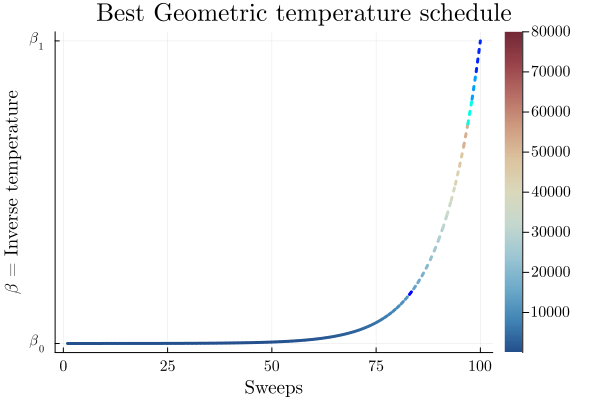
# For the percentile function
# QUBONOTEBOOKS_COLAB_IMPORT_CELL
Base.invokelatest(
    QUBONotebooksBootstrap.load_notebook_packages!,
    "StatsBase",
    :(using StatsBase),
);
println("Calculating optimal sweep...")

schedule_for_min_sweep = primary_schedule

tts_data = results[:ttt][default_sweeps][schedule_for_min_sweep]

finite_tts_data = [
    (t isa Number && isfinite(t)) ? t : Inf
    for t in tts_data
]

min_tts, min_index = findmin(finite_tts_data)

min_sweep = sweeps[min_index]

println("Minimum TTS for '$schedule_for_min_sweep' schedule = $(min_tts)s at sweep = $(min_sweep)")

interest_sweeps = [min_sweep, default_sweeps, comparison_sweeps...]

n_boot_plot = total_reads

schedules_for_plot = [primary_schedule]

boot_range = 1:(total_reads - 1)

approx_ratio = Dict{String, Dict{Int, Vector{Float64}}}()
approx_ratioci = Dict{String, Dict{Int, Vector{Tuple{Float64, Float64}}}}()

p_approx = plot()

for schedule in schedules_for_plot
    approx_ratio[schedule] = Dict{Int, Vector{Float64}}()
    approx_ratioci[schedule] = Dict{Int, Vector{Tuple{Float64, Float64}}}()

    min_energy = results[:min_energy][schedule]
    random_energy = results[:random_energy][schedule]

    for sweep in interest_sweeps
        println("Processing sweep $sweep for schedule $schedule...")

        # Reuse the single-instance cache from the sweep study above.
        solution_name = joinpath(pickle_path, "solutions_$(total_reads)_$(sweep)_$(schedule).json")

        local sol
        if isfile(solution_name) && !overwrite_pickles
            sol = QUBOTools.read_solution(solution_name)
        else
            println("Solution file not found: $solution_name. Re-running simulation.")
            set_attribute(random_ising_model, "num_reads", total_reads)
            set_attribute(random_ising_model, "num_sweeps", sweep)
            set_attribute(random_ising_model, "beta_schedule_type", schedule)

            optimize!(random_ising_model)

            sol = QUBOTools.solution(QUBOTools.backend(random_ising_model))
            open(solution_name, "w") do io
                QUBOTools.write_solution(io, sol, QUBOTools.Format{:bqpjson}())
            end
        end

        energies_unique = QUBOTools.value.(sol)
        occurrences = QUBOTools.reads.(sol)

        all_energies = vcat([fill(energies_unique[i], occurrences[i]) for i in 1:length(energies_unique)]...)

        current_min = minimum(all_energies)
        if current_min < min_energy
            println("A better solution of '$(current_min)' was found for sweep '$sweep'")
            min_energy = current_min
        end

        b = Float64[]
        bcs = Tuple{Float64, Float64}[]

        for boot_size in boot_range
            boot_dist = Float64[]

            for _ in 1:n_boot_plot
                resampler = rand(1:length(all_energies), boot_size)
                sample_boot = all_energies[resampler]

                push!(boot_dist, minimum(sample_boot))
            end

            push!(b, mean(boot_dist))

            cilo = percentile(boot_dist, 50 - ci / 2)
            ciup = percentile(boot_dist, 50 + ci / 2)
            push!(bcs, (cilo, ciup))
        end

        approx_ratio[schedule][sweep] = [
            (random_energy - energy) / (random_energy - min_energy) for energy in b
        ]

        approx_ratioci[schedule][sweep] = [
            ((random_energy - ci_low) / (random_energy - min_energy),
             (random_energy - ci_high) / (random_energy - min_energy))
            for (ci_low, ci_high) in bcs
        ]

        x_values = [shot * sweep for shot in boot_range]
        y_values = approx_ratio[schedule][sweep]

        ci_data = approx_ratioci[schedule][sweep]
        upper_bound_series = getindex.(ci_data, 1)
        lower_bound_series = getindex.(ci_data, 2)

        ribbon_low = y_values .- lower_bound_series
        ribbon_high = upper_bound_series .- y_values

        plot!(p_approx, x_values, y_values,
              label="$sweep sweeps",
              linewidth=2)

        plot!(p_approx, x_values, y_values;
              ribbon=(ribbon_low, ribbon_high),
              fillalpha=0.25,
              label="",
              linewidth=0)
    end
end

title_str = "Simulated annealing Performance Ratio of Ising $(benchmark_instance) N=100\n with varying schedule, $n_boot_plot bootstrap re-samples, and sweeps"
ylabel_str = "Performance Ratio = \n (best found - random sample) / (min energy - random sample)"
xlabel_str = "Total number of reads (equivalent to time)"

plot!(p_approx,
    plot_title = title_str,
    size = (1000, 900),
    xlabel = xlabel_str,
    ylabel = ylabel_str,
    xscale = :log10,
    xticks = 10.0.^(2:4),  # Explicit ticks for log scale to avoid warnings
    ylims = (0.9, 1.01),
    xlims = (1e2, 1e4),
    legend = :bottomright,

    plot_titlevspan = 0.1,
    plot_titlefont  = Plots.font(16, "Computer Modern"),
    guidefont       = Plots.font(12, "Computer Modern"),
    legendfont      = Plots.font(10, "Computer Modern"),
    tickfont        = Plots.font(10, "Computer Modern")
)

display(p_approx)
Here see how using the optimal number of sweeps is better than using other values (including the default recommended by the solver) in terms of solving this problem. Obviously, we only know this after running the experiments and verifying it ourselves. This is not the usual case, so we want to see how well can we do if we solve similar (but no the same instances). Here we will generate 20 random instances from the same distribution and size but different random seed.
println("Starting multi-instance analysis...")

instances = ensemble_instances
schedules_multi = [primary_schedule]

all_results_name = joinpath(pickle_path, "all_results.json")

function metric_raw(raw, julia_name, python_name = julia_name)
    if haskey(raw, julia_name)
        return raw[julia_name]
    end
    return raw[python_name]
end

function has_numeric_keys(raw)
    return all(k -> tryparse(Int, string(k)) !== nothing, keys(raw))
end

function unwrap_default_sweep(raw, default_sweep_count)
    if raw isa AbstractDict && haskey(raw, string(default_sweep_count))
        return raw[string(default_sweep_count)]
    end
    return raw
end

function restore_schedule_dict(raw, default_sweep_count)
    return Dict{String, Any}(string(k) => benchmark_cache_from_json(unwrap_default_sweep(v, default_sweep_count)) for (k, v) in raw)
end

function restore_boot_schedule_dict(raw, default_sweep_count)
    return Dict{Int, Any}(
        parse(Int, string(k)) => restore_schedule_dict(v, default_sweep_count)
        for (k, v) in raw
    )
end

function restore_schedule_boot_dict(raw, default_sweep_count)
    restored = Dict{Int, Any}()
    for (schedule, boot_values) in raw
        for (boot, values) in boot_values
            boot_key = parse(Int, string(boot))
            if !haskey(restored, boot_key)
                restored[boot_key] = Dict{String, Any}()
            end
            restored[boot_key][string(schedule)] = benchmark_cache_from_json(unwrap_default_sweep(values, default_sweep_count))
        end
    end
    return restored
end

function restore_metric_dict(raw, default_sweep_count)
    if has_numeric_keys(raw)
        return restore_boot_schedule_dict(raw, default_sweep_count)
    end
    return restore_schedule_boot_dict(raw, default_sweep_count)
end

function export_schedule_boot_dict(raw)
    exported = Dict{String, Any}()
    for (boot, schedule_values) in raw
        for (schedule, values) in schedule_values
            if !haskey(exported, schedule)
                exported[schedule] = Dict{String, Any}()
            end
            exported[schedule][string(boot)] = benchmark_cache_to_json(values)
        end
    end
    return exported
end

function export_instance_results(raw)
    return Dict{String, Any}(
        "p"             => export_schedule_boot_dict(raw[:p]),
        "tts"           => export_schedule_boot_dict(raw[:ttt]),
        "ttsci"         => export_schedule_boot_dict(raw[:tttci]),
        "best"          => export_schedule_boot_dict(raw[:best]),
        "bestci"        => export_schedule_boot_dict(raw[:bestci]),
        "t"             => benchmark_cache_to_json(raw[:t]),
        "min_energy"    => benchmark_cache_to_json(raw[:min_energy]),
        "random_energy" => benchmark_cache_to_json(raw[:random_energy]),
    )
end

function export_all_results(raw)
    return Dict{String, Any}(string(k) => export_instance_results(v) for (k, v) in raw)
end

function restore_instance_results(raw, default_sweep_count)
    return Dict{Symbol, Any}(
        :p => restore_metric_dict(raw["p"], default_sweep_count),
        :ttt => restore_metric_dict(metric_raw(raw, "ttt", "tts"), default_sweep_count),
        :tttci => restore_metric_dict(metric_raw(raw, "tttci", "ttsci"), default_sweep_count),
        :best => restore_metric_dict(raw["best"], default_sweep_count),
        :bestci => restore_metric_dict(raw["bestci"], default_sweep_count),
        :t => restore_schedule_dict(raw["t"], default_sweep_count),
        :min_energy => restore_schedule_dict(raw["min_energy"], default_sweep_count),
        :random_energy => restore_schedule_dict(raw["random_energy"], default_sweep_count),
    )
end

function restore_all_results(raw, default_sweep_count)
    return Dict{Int, Any}(
        parse(Int, string(k)) => restore_instance_results(v, default_sweep_count)
        for (k, v) in raw
    )
end

if isfile(all_results_name) && !use_raw_data
    println("Loading multi-instance results from $all_results_name...")
    all_results = restore_all_results(JSON.parsefile(all_results_name), default_sweeps)
else
    all_results = Dict{Int, Any}()
    println("Generating new multi-instance results...")

for instance in instances
    println("--- Processing Instance $instance ---")

    all_results[instance] = Dict{Symbol, Any}(
        :p             => Dict{Int,Any}(),
        :min_energy    => Dict{String,Any}(),
        :random_energy => Dict{String,Any}(),
        :ttt           => Dict{Int,Any}(),
        :tttci         => Dict{Int,Any}(),
        :t             => Dict{String,Any}(),
        :best          => Dict{Int,Any}(),
        :bestci        => Dict{Int,Any}(),
    )

    Random.seed!(instance)

    J_instance = triu!(2rand(Float64, n, n) .- 1, 1)
    h_instance = 2rand(Float64, n) .- 1

    instance_model = Model()
    @variable(instance_model, s_inst[1:n], Spin)
    @objective(instance_model, Min, s_inst' * J_instance * s_inst + h_instance' * s_inst)

    set_optimizer(instance_model, QUBO.RandomSampler.Optimizer)
    set_attribute(instance_model, "num_reads", total_reads)
    optimize!(instance_model)

    instance_energies = [objective_value(instance_model; result = i) for i = 1:result_count(instance_model)]
    instance_random_energy = mean(instance_energies)

    # Per-instance cache: the key includes instance because each ensemble member is generated separately.
    default_sol_name = joinpath(pickle_path, "solutions_$(instance)_$(primary_schedule)_$(default_sweeps).json")

    local default_sol

    if isfile(default_sol_name) && !overwrite_pickles
        default_sol = QUBOTools.read_solution(default_sol_name)
    else
        set_optimizer(instance_model, DWave.Neal.Optimizer)
        set_attribute(instance_model, "num_reads", total_reads)
        set_attribute(instance_model, "num_sweeps", default_sweeps)
        set_attribute(instance_model, "beta_schedule_type", primary_schedule)

        optimize!(instance_model)
        default_sol = QUBOTools.solution(QUBOTools.backend(instance_model))

        open(default_sol_name, "w") do io
            QUBOTools.write_solution(io, default_sol, QUBOTools.Format{:bqpjson}())
        end
    end

    default_energies = QUBOTools.value.(default_sol)
    instance_min_energy = minimum(default_energies)

    current_min_energy = instance_min_energy

    for schedule in schedules_multi
        probs       = Dict{Int,Any}(k => [] for k in boots)
        time_to_sol = Dict{Int,Any}(k => [] for k in boots)
        tttcs       = Dict{Int,Any}(k => [] for k in boots)
        times       = []
        b           = Dict{Int,Any}(k => [] for k in boots)
        bcs         = Dict{Int,Any}(k => [] for k in boots)

        for sweep in sweeps
            # Per-instance sweep cache for ensemble timing and success-probability analysis.
            sol_filename = joinpath(pickle_path, "solutions_$(instance)_$(schedule)_$(sweep).json")

            local sol
            local time_s

            if isfile(sol_filename) && !overwrite_pickles
                sol = QUBOTools.read_solution(sol_filename)
                time_s = QUBOTools.total_time(sol)
            else
                set_optimizer(instance_model, DWave.Neal.Optimizer)
                set_attribute(instance_model, "num_reads", total_reads)
                set_attribute(instance_model, "num_sweeps", sweep)
                set_attribute(instance_model, "beta_schedule_type", schedule)

                optimize!(instance_model)

                sol = QUBOTools.solution(QUBOTools.backend(instance_model))
                time_s = QUBOTools.total_time(sol)

                open(sol_filename, "w") do io
                    QUBOTools.write_solution(io, sol, QUBOTools.Format{:bqpjson}())
                end
            end

            energies     = QUBOTools.value.(sol)
            occurrences  = QUBOTools.reads.(sol)

            push!(times, time_s)

            if minimum(energies) < current_min_energy
                current_min_energy = minimum(energies)
                @info("Instance $instance: New min energy '$(current_min_energy)' found for sweep '$sweep'")
            end

            success = instance_random_energy - (instance_random_energy - current_min_energy)*(1.0 - threshold/100.0)

            all_energies_expanded = vcat([fill(energies[i], occurrences[i]) for i in 1:length(energies)]...)

            for boot in boots
                boot_dist = Float64[] # Store min energies
                pr_dist   = Float64[] # Store success probabilities

                for i in 1:n_boot
                    resampler = rand(1:length(all_energies_expanded), boot)
                    sample_boot = all_energies_expanded[resampler]

                    push!(boot_dist, minimum(sample_boot))

                    success_count = count(<(success), sample_boot)
                    push!(pr_dist, success_count / boot)
                end

                push!(b[boot], mean(boot_dist))

                bnp_boot  = boot_dist
                cilo_boot = percentile(bnp_boot, 50 - ci / 2)
                ciup_boot = percentile(bnp_boot, 50 + ci / 2)
                push!(bcs[boot], (cilo_boot, ciup_boot))

                prob_np_boot = pr_dist
                pr_boot      = mean(prob_np_boot)
                if pr_boot >= 1
                    pr_boot = 1 - 1E-9
                end
                push!(probs[boot], pr_boot)

                if !all(x -> x > 0, prob_np_boot)
                    push!(time_to_sol[boot], Inf)
                    push!(tttcs[boot], (Inf, Inf))
                else
                    pr_cilo_boot = percentile(prob_np_boot, 50 - ci / 2)
                    if pr_cilo_boot >= 1
                        pr_cilo_boot = 1 - 1E-9
                    end
                    pr_ciup_boot = percentile(prob_np_boot, 50 + ci / 2)
                    if pr_ciup_boot >= 1
                        pr_ciup_boot = 1 - 1E-9
                    end

                    try
                        push!(time_to_sol[boot], time_s * log10(1-s) / log10(1 - pr_boot + 1E-9))
                        push!(
                             tttcs[boot],
                            (
                                time_s*log10(1-s)/log10(1 - pr_cilo_boot + 1E-9),
                                time_s*log10(1-s)/log10(1 - pr_ciup_boot + 1E-9)
                            )
                        )
                    catch e
                        @warn "Error in TTT calculation for instance $instance, sweep $sweep: $e"
                        push!(time_to_sol[boot], Inf)
                        push!(tttcs[boot], (Inf, Inf))
                    end
                end
            end
        end

        all_results[instance][:t][schedule]             = times
        all_results[instance][:min_energy][schedule]    = current_min_energy
        all_results[instance][:random_energy][schedule] = instance_random_energy

        for boot in boots
            if !haskey(all_results[instance][:p], boot)
                all_results[instance][:p][boot] = Dict{String, Any}()
            end

            all_results[instance][:p][boot][schedule] = probs[boot]

            if !haskey(all_results[instance][:ttt], boot)
                all_results[instance][:ttt][boot] = Dict{String, Any}()
            end
            all_results[instance][:ttt][boot][schedule]   = time_to_sol[boot]

            if !haskey(all_results[instance][:tttci], boot)
                all_results[instance][:tttci][boot] = Dict{String, Any}()
            end
            all_results[instance][:tttci][boot][schedule] = tttcs[boot]

            if !haskey(all_results[instance][:best], boot)
                all_results[instance][:best][boot] = Dict{String, Any}()
            end
            all_results[instance][:best][boot][schedule]  = [
                (instance_random_energy - energy) / (instance_random_energy - current_min_energy)
                for energy in b[boot]
            ]

            if !haskey(all_results[instance][:bestci], boot)
                all_results[instance][:bestci][boot] = Dict{String, Any}()
            end
            all_results[instance][:bestci][boot][schedule] = [
                tuple(((instance_random_energy - element) / (instance_random_energy - current_min_energy) for element in energy)...)
                for energy in bcs[boot]
            ]
        end
    end
end

println("Saving multi-instance results to $all_results_name...")
open(all_results_name, "w") do io
    JSON.print(io, export_all_results(all_results))
end
println("Save complete.")
end

println("Multi-instance analysis script finished.")
Starting multi-instance analysis...
Loading multi-instance results from <notebook-directory>/results/all_results.json...
Multi-instance analysis script finished.
# zip the processed benchmark summaries
zip_name = joinpath(pickle_path, "results.zip")
processed_result_file_names = [
    file_name
    for file_name in sort(readdir(pickle_path))
    if isfile(joinpath(pickle_path, file_name)) &&
       abspath(joinpath(pickle_path, file_name)) != abspath(zip_name) &&
       (file_name == "all_results.json" || (startswith(file_name, "results_") && endswith(file_name, ".json")))
]
archive_size_limit = typemax(UInt32)
archive_size_bytes = sum(filesize(joinpath(pickle_path, file_name)) for file_name in processed_result_file_names; init = 0)

if archive_size_bytes > archive_size_limit
    @warn "Skipping results.zip archive because the processed result set is $(archive_size_bytes) bytes and ZipFile does not support ZIP64 archives."
else
    w = ZipFile.Writer(zip_name)

    try
        for file_name in processed_result_file_names
            file_path = joinpath(pickle_path, file_name)
            f = ZipFile.addfile(w, file_name)
            write(f, read(file_path))
        end
    finally
        close(w)
    end
end
"""
Calculates the median of an array, skipping NaN values.
`dims=1` calculates the median for each column (across instances).
`dims=2` calculates the median for each row (across sweeps).
"""
function nanmedian(A; dims)
    return mapslices(A, dims=dims) do v
        filtered_v = filter(!isnan, v)
        return isempty(filtered_v) ? NaN : median(filtered_v)
    end
end

"""
Calculates the standard deviation of an array, skipping NaN values.
"""
function nanstd(A; dims)
    return mapslices(A, dims=dims) do v
        filtered_v = filter(!isnan, v)
        return isempty(filtered_v) ? NaN : std(filtered_v)
    end
end

finite_or_nan_vec(raw_vec) = [
    (v isa Number && isfinite(v)) ? v : NaN
    for v in raw_vec
]

finite_or_inf_vec(raw_vec) = [
    (v isa Number && isfinite(v)) ? v : Inf
    for v in raw_vec
]

finite_or_nan(val) = (val isa Number && isfinite(val)) ? val : NaN

function ensemble_ttt_matrix(all_results, instances, boot, schedule)
    return vcat([
        transpose(finite_or_nan_vec(all_results[i][:ttt][boot][schedule]))
        for i in instances
    ]...)
end

function min_median_ttt(all_results, instances, boot, schedule)
    results_array = ensemble_ttt_matrix(all_results, instances, boot, schedule)
    median_tts = nanmedian(results_array, dims=1)[1,:]
    min_median_tts, min_median_index = findmin(finite_or_inf_vec(median_tts))

    return (
        results_array = results_array,
        median_tts = median_tts,
        min_median_tts = min_median_tts,
        min_median_index = min_median_index,
    )
end

"""
Performs bootstrapping to find the confidence interval of the median.
"""
function bootstrap(data; n_boot=1000, ci=68)
    boot_dist = []

    n_instances = size(data, 1) # Number of rows (instances)

    for i in 1:n_boot
        resampler_idx = rand(1:n_instances, n_instances)
        sample = data[resampler_idx, :]

        push!(boot_dist, nanmedian(sample, dims=1))
    end

    b = vcat(boot_dist...)

    s1 = mapslices(b, dims=1) do v
        filtered_v = filter(!isnan, v)
        return isempty(filtered_v) ? NaN : percentile(filtered_v, 50.0 - ci/2.0)
    end

    s2 = mapslices(b, dims=1) do v
        filtered_v = filter(!isnan, v)
        return isempty(filtered_v) ? NaN : percentile(filtered_v, 50.0 + ci/2.0)
    end

    return (s1, s2)
end

"""
Plots a time series (median) with a shaded confidence interval (ribbon).
"""
function tsplotboot!(plt, x, data, error_est; label="", kwargs...)
    est = nanmedian(data, dims=1)[1,:]

    mask = .!isnan.(est)
    x_masked = x[mask]
    est_masked = est[mask]

    local ci_low, ci_high
    if error_est == "bootstrap"
        cis = bootstrap(data)
        ci_low = cis[1][1,:][mask] # [1,:] to get 1D Vector
        ci_high = cis[2][1,:][mask]
    elseif error_est == "std"
        sd = nanstd(data, dims=1)[1,:][mask]
        ci_low = est_masked .- sd
        ci_high = est_masked .+ sd
    end

    ribbon_low = est_masked .- ci_low
    ribbon_high = ci_high .- est_masked

    plot!(plt, x_masked, est_masked;
          right_margin  = 30mm,
          left_margin   = 10mm,
          ribbon=(ribbon_low, ribbon_high),
          fillalpha=0.35,
          label=label,
          kwargs...)
endtsplotboot!Now we bootstrap our solutions across the full set of instances, or ensemble, and use the median because it is less sensitive to outliers than the mean.
plt = plot(
    size = (1000, 800),
    title = "Simulated annealing expected total runtime of \n Ising $(benchmark_instance) N=100 with varying schedule and sweeps",
    yscale = :log10,
    yticks = 10.0.^(-2:1),  # Explicit ticks for log scale to avoid warnings
    ylabel = "Total Time To Solution within $threshold % of best found [s]",
    xlabel = "Sweeps",
    legend = :outerbottom,
    legend_columns = 3
)

schedules_to_plot = [primary_schedule]
inset_padding = 5

for boot in reverse(boots)
    for schedule in schedules_to_plot
        results_array = ensemble_ttt_matrix(all_results, instances, boot, schedule)

        tsplotboot!(plt, sweeps, results_array, "bootstrap";
                    label="Ensemble $schedule with $boot reads")

        clean_vec_benchmark = finite_or_nan_vec(results[:ttt][boot][schedule])
        plot!(plt, sweeps, clean_vec_benchmark;
              label="Instance $(benchmark_instance) $(schedule)_boot$boot")
    end
end

plot!(plt,
    inset = (1, bbox(0.2, 0.0, 0.4, 0.3)),
    subplot = 2,
    yscale = :log10,
    yticks = 10.0.^(-2:1),  # Explicit ticks for log scale to avoid warnings
    ylabel = "Total TTS [s]",
    xlabel = "Sweeps",
    framestyle = :box,
    legend = false,
    tickfont = Plots.font(8, "Computer Modern")
)

median_summary_by_schedule = Dict{String, Any}()

for schedule in schedules_to_plot
    inset_summary = min_median_ttt(all_results, instances, default_sweeps, schedule)
    median_summary_by_schedule[schedule] = inset_summary

    median_tts_inset = inset_summary.median_tts
    schedule_min_median_index = inset_summary.min_median_index
    min_median_tts_val = inset_summary.min_median_tts
    schedule_min_median_sweep = sweeps[schedule_min_median_index]

    clean_vec_benchmark_inset = finite_or_nan_vec(results[:ttt][default_sweeps][schedule])
    min_tts_benchmark_val, min_index_benchmark = findmin(finite_or_inf_vec(clean_vec_benchmark_inset))
    min_sweep_benchmark = sweeps[min_index_benchmark]

    index_lo, index_hi = sort([min_index_benchmark, schedule_min_median_index])
    range_lo = max(1, index_lo - inset_padding)
    range_hi = min(length(sweeps), index_hi + inset_padding)
    plot_range = range_lo:range_hi

    println("minimum median TTS for $schedule schedule = $min_median_tts_val s at sweep = $schedule_min_median_sweep")
    println("minimum TTS for instance $benchmark_instance with $schedule schedule = $min_tts_benchmark_val s at sweep = $min_sweep_benchmark")

    plot!(plt[2], sweeps[plot_range], median_tts_inset[plot_range],
          linestyle=:solid, marker=:square, label="")

    plot!(plt[2], sweeps[plot_range], clean_vec_benchmark_inset[plot_range],
          linestyle=:solid, marker=:square, label="")

    default_vals = [
        let v = all_results[i][:ttt][default_sweeps][schedule][end]
            finite_or_nan(v)
        end
        for i in instances
    ]
    median_default = nanmedian(default_vals, dims=1)[1]

    hline!(plt[2], [median_default],
           linestyle=:dash, color=:blue, label="")
end

primary_median_summary = median_summary_by_schedule[primary_schedule]
min_median_index = primary_median_summary.min_median_index
min_median_sweep = sweeps[min_median_index]

display(plt)
plt_approx = plot(
size = (1000, 800),
plot_title = "Simulated annealing Performance Ratio of \n Ensemble of Ising N=100 with varying schedule, sweeps, and number of reads",
xlabel = "Sweeps",
ylabel = "Performance Ratio = \n (best found - random sample) / (min energy - random sample)",
xscale = :log10,
xticks = 10.0.^(0:3), # Explicit ticks for log scale to avoid warnings
ylims = (0.8, 1.01),
legend = :outerbottom,
legend_columns = 3,
plot_titlevspan = 0.1,
plot_titlefont = Plots.font(16, "Computer Modern"),
guidefont = Plots.font(12, "Computer Modern"),
legendfont = Plots.font(10, "Computer Modern"),
tickfont = Plots.font(10, "Computer Modern")
)
schedules_to_plot = [primary_schedule]
for boot in boots
for schedule in schedules_to_plot
data_list = []
for i in instances
raw_vec = all_results[i][:best][boot][schedule]
clean_vec = [v isa Number ? (isfinite(v) ? v : NaN) : NaN for v in raw_vec]
push!(data_list, transpose(clean_vec))
end
best_array = vcat(data_list...)
tsplotboot!(plt_approx, sweeps, best_array, "bootstrap";
label="Ensemble $schedule with $boot reads",
linewidth=2)
end
end
display(plt_approx)plt_total_reads = plot(
size = (1000, 800),
plot_title = "Simulated annealing Performance Ratio of \n Ensemble of Ising N=100 with varying schedule, sweeps, and number of reads",
xlabel = "Total number of reads",
ylabel = "Performance Ratio = \n (best found - random sample) / (min energy - random sample)",
xscale = :log10,
xticks = 10.0.^(2:5), # Explicit ticks for log scale to avoid warnings
ylims = (0.8, 1.01),
legend = :outerbottom,
legend_columns = 3,
plot_titlevspan = 0.1,
plot_titlefont = Plots.font(16, "Computer Modern"),
guidefont = Plots.font(12, "Computer Modern"),
legendfont = Plots.font(10, "Computer Modern"),
tickfont = Plots.font(10, "Computer Modern")
)
schedules_to_plot = [primary_schedule]
for boot in boots
reads = [s * boot for s in sweeps]
for schedule in schedules_to_plot
data_list = []
for i in instances
raw_vec = all_results[i][:best][boot][schedule]
clean_vec = [v isa Number ? (isfinite(v) ? v : NaN) : NaN for v in raw_vec]
push!(data_list, transpose(clean_vec))
end
best_array = vcat(data_list...)
tsplotboot!(plt_total_reads, reads, best_array, "bootstrap";
label="Ensemble $schedule with $boot reads",
linewidth=2)
end
end
display(plt_total_reads)median_summary = min_median_ttt(all_results, instances, default_sweeps, primary_schedule)
min_median_val = median_summary.min_median_tts
min_median_index = median_summary.min_median_index
raw_tts_vectors = [all_results[i][:ttt][default_sweeps][primary_schedule] for i in instances]
cleaned_tts_vectors = [finite_or_inf_vec(v) for v in raw_tts_vectors]
minima = [minimum(v) for v in cleaned_tts_vectors]
median_all = [finite_or_nan(v[min_median_index]) for v in raw_tts_vectors]
default = [finite_or_nan(v[end]) for v in raw_tts_vectors]
plt_bar = plot(
size = (700, 500),
xlabel = "Instance",
ylabel = "Total Time To Solution within $threshold % of best found [s]",
legend = :top,
plot_titlefont = Plots.font(16, "Computer Modern"),
guidefont = Plots.font(12, "Computer Modern"),
legendfont = Plots.font(10, "Computer Modern"),
tickfont = Plots.font(10, "Computer Modern")
)
bar!(plt_bar, instances .- 0.2, minima,
bar_width=0.2, label="virtual best", color=:blue)
bar!(plt_bar, instances, median_all,
bar_width=0.2, label="median", color=:green)
bar!(plt_bar, instances .+ 0.2, default,
bar_width=0.2, label="default", color=:red)
plot!(plt_bar, xticks = instances)
display(plt_bar)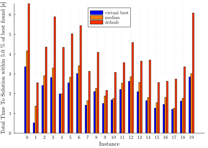
Notice how much performance would we be losing if we had used the default value for all these instances, and how much we could eventually win if we knew the best for each.
println("Calculating optimal sweep for instance $benchmark_instance...")
tts_data_benchmark = results[:ttt][default_sweeps][primary_schedule]
finite_tts_data_benchmark = [
    (t isa Number && isfinite(t)) ? t : Inf
    for t in tts_data_benchmark
]
min_tts_benchmark, min_index_benchmark = findmin(finite_tts_data_benchmark)
min_sweep = sweeps[min_index_benchmark]

min_median_sweep = sweeps[min_median_index]

println("Minimum TTS for instance $benchmark_instance = $(min_tts_benchmark)s at sweep = $(min_sweep)")
println("Minimum MEDIAN TTS (all instances) at sweep = $(min_median_sweep)")

interest_sweeps = [min_sweep, default_sweeps, comparison_sweeps..., min_median_sweep]
interest_sweeps = unique(interest_sweeps)

n_boot_plot = total_reads
schedules_for_plot = [primary_schedule]
boot_range = 1:(total_reads - 1)

approx_ratio = Dict{String, Dict{Int, Vector{Float64}}}()
approx_ratioci = Dict{String, Dict{Int, Vector{Tuple{Float64, Float64}}}}()

p_approx = plot()

for schedule in schedules_for_plot
    approx_ratio[schedule] = Dict{Int, Vector{Float64}}()
    approx_ratioci[schedule] = Dict{Int, Vector{Tuple{Float64, Float64}}}()

    min_energy = results[:min_energy][schedule]
    random_energy = results[:random_energy][schedule]

    for sweep in interest_sweeps
        println("Processing sweep $sweep for schedule $schedule...")

        # Benchmark-instance cache: this key includes instance to match the ensemble cache schema.
        sol_filename = joinpath(pickle_path, "solutions_$(instance)_$(schedule)_$(sweep).json")

        local sol
        if isfile(sol_filename) && !overwrite_pickles
            sol = QUBOTools.read_solution(sol_filename)
        else
            println("Solution file not found: $sol_filename. Re-running simulation.")
            set_optimizer(random_ising_model, DWave.Neal.Optimizer)
            set_attribute(random_ising_model, "num_reads", total_reads)
            set_attribute(random_ising_model, "num_sweeps", sweep)
            set_attribute(random_ising_model, "beta_schedule_type", schedule)

            optimize!(random_ising_model)
            sol = QUBOTools.solution(QUBOTools.backend(random_ising_model))

            open(sol_filename, "w") do io
                QUBOTools.write_solution(io, sol, QUBOTools.Format{:bqpjson}())
            end
        end

        energies_unique = QUBOTools.value.(sol)
        occurrences = QUBOTools.reads.(sol)

        all_energies = vcat([fill(energies_unique[i], occurrences[i]) for i in 1:length(energies_unique)]...)

        current_min = isempty(all_energies) ? Inf : minimum(all_energies)
        if current_min < min_energy
            println("A better solution of '$(current_min)' was found for sweep '$sweep'")
            min_energy = current_min
        end

        b = Float64[]
        bcs = Tuple{Float64, Float64}[]

        for boot_size in boot_range
            shot_dist = Float64[]

            for _ in 1:n_boot_plot
                resampler = rand(1:length(all_energies), boot_size)
                sample_boot = all_energies[resampler]

                push!(shot_dist, minimum(sample_boot))
            end

            push!(b, mean(shot_dist))

            bnp = filter(!isnan, shot_dist)
            if isempty(bnp)
                push!(bcs, (NaN, NaN))
            else
                cilo = percentile(bnp, 50 - ci / 2)
                ciup = percentile(bnp, 50 + ci / 2)
                push!(bcs, (cilo, ciup))
            end
        end

        approx_ratio[schedule][sweep] = [
            (random_energy - energy) / (random_energy - min_energy) for energy in b
        ]

        approx_ratioci[schedule][sweep] = [
            (
                (random_energy - ci_low) / (random_energy - min_energy),
                (random_energy - ci_high) / (random_energy - min_energy)
            )
            for (ci_low, ci_high) in bcs
        ]

        x_values = [shot * sweep for shot in boot_range]
        y_values = approx_ratio[schedule][sweep]


        ci_data = approx_ratioci[schedule][sweep]
        upper_bound_series = getindex.(ci_data, 1)
        lower_bound_series = getindex.(ci_data, 2)

        ribbon_low = y_values .- lower_bound_series
        ribbon_high = upper_bound_series .- y_values

        plot!(p_approx, x_values, y_values,
              label="$sweep sweeps",
              linewidth=2,
              ribbon=(ribbon_low, ribbon_high),
              fillalpha=0.25)
    end
end


title_str = "Simulated annealing Performance Ratio of Ising $(benchmark_instance) N=100\n with varying schedule, $n_boot_plot bootstrap re-samples, and sweeps"
ylabel_str = "Performance Ratio = \n (best found - random sample) / (min energy - random sample)"
xlabel_str = "Total number of reads (equivalent to time)"

plot!(p_approx,
    plot_title = title_str,
    xlabel = xlabel_str,
    ylabel = ylabel_str,
    xscale = :log10,
    xticks = 10.0.^(2:4),  # Explicit ticks for log scale to avoid warnings
    ylims = (0.95, 1.001),
    xlims = (1e2, 1e4),
    legend = :best,

    size = (700, 600),
    plot_titlevspan = 0.1,
    plot_titlefont  = Plots.font(14, "Computer Modern"),
    guidefont       = Plots.font(12, "Computer Modern"),
    legendfont      = Plots.font(10, "Computer Modern"),
    tickfont        = Plots.font(10, "Computer Modern")
)

display(p_approx)
This example shows that for the benchmark instance, using the mean of the best accross the ensemble is better than using the default, but not as good as if we knew from scratch what would have made the best case.
After figuring out what would be the best parameter for our instance of interest, it would be nice to see what the ensemble performance is. We have several choices, either going with the (arbitrary) default values, or using the mean of the best performance we have found up to that point. There is an unachievable goal, which would be the case where we knew the best solution of each case, which we call the virtual best. This helps us understand how much is at stake with the choice of parameters we make.
n_boot_plot = 100
schedules_for_plot = [primary_schedule]
boot_range = 1:(total_reads - 1)
overwrite_pickles = false

indices = Int[]
for i in instances
    raw_vec = all_results[i][:ttt][default_sweeps][primary_schedule]
    push!(indices, argmin(finite_or_inf_vec(raw_vec)))
end

min_median_sweep = sweeps[min_median_index]
interest_sweeps_keys = [string(min_median_sweep), string(default_sweeps), "best"]

all_approx_ratio = Dict{Int, Dict{String, Dict{String, Any}}}()
for instance in instances
    all_approx_ratio[instance] = Dict{String, Dict{String, Any}}()
    for schedule in schedules_for_plot
        all_approx_ratio[instance][schedule] = Dict{String, Any}()
    end
end

plt_final = plot(
    size = (700, 600),
    title = "Simulated annealing Performance Ratio of Ising Ensemble N=100\n with varying schedule, $n_boot_plot bootstrap re-samples, and sweeps",
    xlabel = "Total number of reads (equivalent to time)",
    ylabel = "Performance Ratio = \n (best found - random sample) / (min energy - random sample)",
    xscale = :log10,
    xticks = 10.0.^(2:4),  # Explicit ticks for log scale to avoid warnings
    ylims = (0.95, 1.001),
    xlims = (1e2, 1e4),

    legend = :best,
    plot_titlevspan = 0.1,
    plot_titlefont  = Plots.font(14, "Computer Modern"),
    guidefont       = Plots.font(10, "Computer Modern"),
    legendfont      = Plots.font(10, "Computer Modern"),
    tickfont        = Plots.font(10, "Computer Modern")
)

for instance in instances
    println("Processing instance $instance...")

    Random.seed!(instance)
    J_instance = triu!(2rand(Float64, n, n) .- 1, 1)
    h_instance = 2rand(Float64, n) .- 1

    instance_model = Model()
    @variable(instance_model, s_inst[1:n], Spin)
    @objective(instance_model, Min, s_inst' * J_instance * s_inst + h_instance' * s_inst)
    set_optimizer(instance_model, DWave.Neal.Optimizer)

    for sweep_key in interest_sweeps_keys
        flag_best = false
        current_sweep = 0

        if sweep_key == "best"
            flag_best = true
            current_sweep = sweeps[indices[instance + 1]]
        else
            current_sweep = parse(Int, sweep_key)
        end

        schedule = primary_schedule

        min_energy = all_results[instance][:min_energy][primary_schedule]
        random_energy = all_results[instance][:random_energy][primary_schedule]

        # Per-instance approx-ratio cache for selected sweeps and best-sweep comparisons.
        sol_filename = joinpath(pickle_path, "solutions_$(instance)_$(schedule)_$(current_sweep).json")

        local sol
        if isfile(sol_filename) && !overwrite_pickles
            sol = QUBOTools.read_solution(sol_filename)
        else
            set_attribute(instance_model, "num_reads", total_reads)
            set_attribute(instance_model, "num_sweeps", current_sweep)
            set_attribute(instance_model, "beta_schedule_type", schedule)

            optimize!(instance_model)
            sol = QUBOTools.solution(QUBOTools.backend(instance_model))

            open(sol_filename, "w") do io
                QUBOTools.write_solution(io, sol, QUBOTools.Format{:bqpjson}())
            end
        end

        energies_unique = QUBOTools.value.(sol)
        occurrences = QUBOTools.reads.(sol)
        all_energies = vcat([fill(energies_unique[i], occurrences[i]) for i in 1:length(energies_unique)]...)

        current_min = isempty(all_energies) ? Inf : minimum(all_energies)
        if current_min < min_energy
            min_energy = current_min
        end

        b = Float64[]

        for boot_size in boot_range
            shot_dist = Float64[]
            # Repetitions are independent of the number of reads per resample.
            for _ in 1:n_boot_plot
                resampler = rand(1:length(all_energies), boot_size)
                sample_boot = all_energies[resampler]
                push!(shot_dist, minimum(sample_boot))
            end

            push!(b, mean(shot_dist))
        end

        approx_ratios_vec = [(random_energy - energy) / (random_energy - min_energy) for energy in b]
        plot_key = flag_best ? "best" : sweep_key
        all_approx_ratio[instance][schedule][plot_key] = approx_ratios_vec

        x_values = [shot * current_sweep for shot in boot_range]
        alpha_val = flag_best ? 0.7 : 0.5
        plot!(plt_final, x_values, approx_ratios_vec,
              color=:lightgray, label="", alpha=alpha_val, linewidth=0.7)

    end
end
Processing instance 0...
Processing instance 1...
Processing instance 2...
Processing instance 3...
Processing instance 4...
Processing instance 5...
Processing instance 6...
Processing instance 7...
Processing instance 8...
Processing instance 9...
Processing instance 10...
Processing instance 11...
Processing instance 12...
Processing instance 13...
Processing instance 14...
Processing instance 15...
Processing instance 16...
Processing instance 17...
Processing instance 18...
Processing instance 19...
println("Plotting ensemble data...")
for sweep_key in interest_sweeps_keys
    schedule = primary_schedule

    approx_ratio_array = vcat([
        transpose(all_approx_ratio[i][schedule][sweep_key])
        for i in instances
    ]...)

    label_plot = ""
    current_sweep_for_x = 0

    if sweep_key == "best"
        label_plot = "Ensemble $schedule with virtual best sweeps"
        current_sweep_for_x = sweeps[indices[end]]
    else
        current_sweep_for_x = parse(Int, sweep_key)
        label_plot = "Ensemble $schedule with $sweep_key sweeps"
    end

    reads = [shot * current_sweep_for_x for shot in boot_range]

    tsplotboot!(plt_final, reads, approx_ratio_array, "bootstrap";
                label=label_plot, linewidth=2)
end

display(plt_final)
Plotting ensemble data...
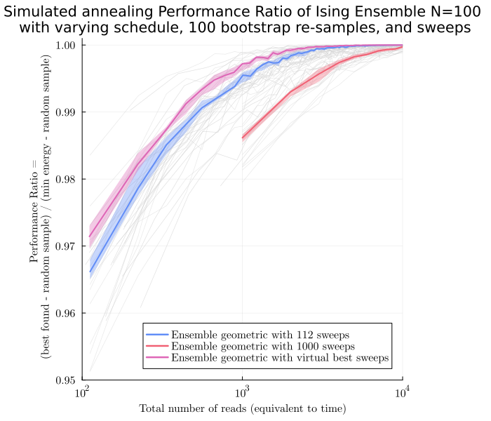
As you can see, there is a gap between the case with the best mean performance and the virtual best. This difference is arguably small, but you can imagine that with a larger number of parameters, this difference can become larger and larger, making the search of good parameters more worthy and complicated. We are actively working on such parameter setting strategies, and expect to make progress in this area (keep tuned!).
Practice checkpoints
Use these checkpoints during the workshop to test the main ideas before moving on.
# =============================================================================
# EXERCISE 1: Add one solver to the comparison
# =============================================================================
# Add a solver or sampler configuration to the existing benchmarking table. Record the same metrics used for the baseline solvers so the comparison is fair.
#
# Hint: Reuse the cache helpers if the run is long.
#
# Your code here:
# =============================================================================
Notebook Cell
# SOLUTION (hidden in workshop version):
# Add a new solver label to a compact benchmarking summary.
solver_results = Dict(
    "baseline_sa" => Dict("best_energy" => -12.4, "time" => 1.8),
    "new_sampler" => Dict("best_energy" => -12.6, "time" => 2.1),
)
sorted_results = sort(collect(solver_results); by = item -> item[2]["best_energy"])
formatted_results = [
    begin
        best_energy = metrics["best_energy"]
        time_value = metrics["time"]
        "$(name): best_energy=$(best_energy), time=$(time_value)"
    end
    for (name, metrics) in sorted_results
]
println("solver_results = $(join(formatted_results, "; "))")
solver_results = new_sampler: best_energy=-12.6, time=2.1; baseline_sa: best_energy=-12.4, time=1.8
# =============================================================================
# EXERCISE 2: Change the success threshold
# =============================================================================
# Compute time-to-solution using a stricter or looser solution-quality threshold. Explain how the threshold changes solver ranking.
#
# Hint: Keep the bootstrapping procedure unchanged so only the success definition changes.
#
# Your code here:
# =============================================================================
Notebook Cell
# SOLUTION (hidden in workshop version):
# Recompute time-to-solution for a changed success threshold.
success_probability = 0.15
target_confidence = 0.99
reads_per_run = 100
tts_reads = ceil(Int, log(1 - target_confidence) / log(1 - success_probability)) * reads_per_run
println("target_confidence = $(target_confidence); tts_reads = $(tts_reads)")
target_confidence = 0.99; tts_reads = 2900
# =============================================================================
# EXERCISE 3: Interpret performance ratio
# =============================================================================
# Choose one instance and explain why its performance-ratio curve differs from another solver or schedule. Connect the plot shape to best, random, and observed energies.
#
# Hint: Identify where the curve is flat, steep, or noisy.
#
# Your code here:
# =============================================================================
Notebook Cell
# SOLUTION (hidden in workshop version):
# Compute a performance ratio from best, random, and observed energies.
best_energy = -15.0
random_energy = -3.0
observed_energy = -12.0
performance_ratio = (observed_energy - random_energy) / (best_energy - random_energy)
println("performance_ratio = $(performance_ratio)")
performance_ratio = 0.75
Summary
In this notebook we:
Treated a solver as a combination of hardware, algorithm, software, and hyperparameters to make comparisons reproducible.
Loaded or generated benchmark samples and converted raw sampling results into success probabilities and time-to-solution metrics.
Used bootstrap summaries and performance ratios to compare schedules, sweeps, default choices, and virtual-best behavior.
Interpreted how tuning on one instance or ensemble can improve results while still leaving a gap to per-instance best choices.
Learning objectives met: You practiced setting up benchmark ensembles, computing TTS and performance ratios, using bootstrap summaries, and interpreting scaling and tuning tradeoffs.
Next steps: Proceed to Python Notebook 6: QCi if you want to compare these benchmarking ideas with a QCi solver workflow.
Further reading:
David E. Bernal Neira — Davidson School of Chemical Engineering, Purdue University
Pedro Maciel Xavier — Davidson School of Chemical Engineering, Purdue University
João Victor Souza — Computer Engineering Department, Military Institute of Engineering (IME)
Acknowledgments
This notebook was developed by:
- Rønnow, T. F., Wang, Z., Job, J., Boixo, S., Isakov, S. V., Wecker, D., Martinis, J. M., Lidar, D. A., & Troyer, M. (2014). Defining and detecting quantum speedup. Science, 345(6195), 420–424. 10.1126/science.1252319