
Setup
Google Colab
Click the badge above. The hidden setup cell installs the QCi stack and HiGHS.
Local installation
From the repository root, use the isolated, locked QCi environment:
uv sync --locked --project notebooks_py/environments/qci
uv run --locked --project notebooks_py/environments/qci jupyter lab
Choose the Python kernel from this environment. For a fresh-kernel check of the
whole notebook, run make verify-qci-python-local from the repository root.
The local path needs no QCi account or separately installed solver binaries.
Cloud examples require an explicit QUBONOTEBOOKS_QCI_ENABLE_CLOUD=1 opt-in and
QCI_TOKEN. Published cloud results are retained historical examples; default
execution skips submissions and their result displays, while constructing and
validating every model locally. Verification writes new results to .nbverify/.
Learning objectives
By the end of this notebook you will be able to:
Describe how QCi’s Dirac solvers represent constrained optimization problems.
Formulate a constrained quadratic or polynomial model with objective coefficients and linear constraints.
Submit a model to Dirac-3 solvers when credentials are available and decode returned solutions.
Compare manual QUBO penalty construction with
ConstrainedPolynomialModelhandling of constraints and offsets.
Prerequisites
Mathematical background: Binary optimization, QUBO penalties, matrix multiplication, and linear equality constraints.
Prior notebooks: Notebook 2 (QUBO) and Notebook 5 (Benchmarking) for solver comparison context.
Accounts required: QCi account credentials and an API token for cloud solver execution.
Python version: Python 3.11–3.12 with the isolated QCi environment.
This notebook provides an introduction to solving constrained optimization problems using Quantum Computing Inc.'s (QCI) Entropy Quantum Computer. We will define a Constrained Quadratic Model by setting up an objective function and a series of linear constraints. The notebook demonstrates how to:
Structure the problem using QCI’s
eqc_modelslibrary.Submit the model to the
Dirac3IntegerCloudSolverandDirac3ContinuousSolverfor processing.Analyze the high-quality candidate solutions returned by the solver to find the optimal result.
Notebook Cell
# Install the isolated QCi stack only in a hosted Colab runtime.
try:
    import google.colab
    IN_COLAB = True
except ImportError:
    IN_COLAB = False

if IN_COLAB:
    import subprocess
    import sys

    subprocess.run([
        sys.executable, "-m", "pip", "install", "-q", "eqc-models==0.20.2",
        "highspy>=1.15.1,<2", "pyomo>=6.9,<7", "matplotlib>=3.8,<4", "numpy>=1.26,<3",
    ], check=True)
# eqc-models 0.20.2 omits its optional direct-hardware client on Python 3.11+.
# Suppress only that exact import-time log; cloud clients remain available.
import logging


class OptionalDirectSolverNotice(logging.Filter):
    def filter(self, record):
        return not (
            record.name == "root"
            and record.levelno == logging.WARNING
            and record.getMessage() == "eqc-direct package not available"
            and record.pathname.replace("\\", "/").endswith("/eqc_models/solvers/eqcdirect.py")
        )


_direct_notice = OptionalDirectSolverNotice()
logging.getLogger().addFilter(_direct_notice)
try:
    import eqc_models
    from eqc_models.base import ConstrainedPolynomialModel, PolynomialModel, QuadraticModel
    from eqc_models.base.operators import Polynomial
    from eqc_models.solvers import Dirac3IntegerCloudSolver, Dirac3ContinuousCloudSolver
finally:
    logging.getLogger().removeFilter(_direct_notice)

# Import Matplotlib to generate plots
import matplotlib.pyplot as plt
import matplotlib.ticker as mticker

# Import numpy and scipy for certain numerical calculations below
import numpy as np
import pyomo.environ as pyo
import itertools
import io
import os
import warnings
from contextlib import redirect_stderr, redirect_stdout

warnings.filterwarnings(
    "ignore",
    message="Cannot evaluate objective value in results.*",
    category=UserWarning,
)


def solve_without_provider_identifiers(solver, model, **kwargs):
    """Submit a QCI job without publishing provider job or file identifiers."""
    with redirect_stdout(io.StringIO()), redirect_stderr(io.StringIO()):
        response = solver.solve(model, **kwargs)
    print("QCI job completed; provider identifiers are omitted from notebook output.")
    return response


class ScalarConstrainedPolynomialModel(ConstrainedPolynomialModel):
    @staticmethod
    def _scalar(value):
        return float(np.asarray(value).reshape(-1)[0])

    def evaluateObjective(self, solution):
        return self._scalar(super().evaluateObjective(solution))

    def evaluatePenalties(self, solution, include_offset=False):
        coefficients, indices = self.penalties
        value = self.offset if include_offset else 0
        value += self._scalar(
            Polynomial(coefficients, indices).evaluate(
                np.array(solution, dtype=np.float64)
            )
        )
        return float(value)
WARNING:root:eqc-direct package not available
Notebook Cell
# HiGHS handles both the convex quadratic and binary linear references.
if not pyo.SolverFactory("highs").available(exception_flag=False):
    raise RuntimeError("HiGHS is missing. Install the locked QCi environment above.")
How Dirac-3 Works
The Dirac-3 solver is a cloud-based quantum solver that uses the Entropy Quantum Computer (EQC) to solve optimization problems. It encodes a problem into the physical properties of coherent light pulses, allowing it to represent and explore many potential solutions at once within its optical circuits. A controlled feedback loop, managed by electronics, interacts with the light to steer the system away from poor solutions. This process rapidly converges the system onto the single, lowest-energy state, which represents the optimal answer.
QCI API token
QCi cloud execution is an explicit opt-in. Set
QUBONOTEBOOKS_QCI_ENABLE_CLOUD=1 before running the notebook, then provide
QCI_TOKEN through your shell environment or a Colab Secret. A token alone
never enables submission; the default path does not read Colab Secrets.
In Colab, opt in with os.environ["QUBONOTEBOOKS_QCI_ENABLE_CLOUD"] = "1"
before running the next cell. Sign in to the QCi portal to obtain a token.
Missing credentials or an opted-in submission failure stop execution.
api_url = "https://api.qci-prod.com"
enable_qci_cloud = os.environ.get("QUBONOTEBOOKS_QCI_ENABLE_CLOUD", "0") == "1"
api_token = ""
if enable_qci_cloud:
    api_token = os.environ.get("QCI_TOKEN", "")
    if IN_COLAB and not api_token:
        from google.colab import userdata

        api_token = userdata.get("QCI_TOKEN") or ""
    if not api_token:
        raise RuntimeError("Set QCI_TOKEN before opting into QCi cloud execution.")
else:
    print("QCi cloud disabled; all model construction and local checks will run.")
Solving Problems using Dirac-3
Dirac-3 can solve combinatorial optimization problems using the following objective function, E, that has the following high-order polynomial structure:
refers to the value of nonnegative variable, and , , , , and are the coefficients of the objective function. The solver defaults to minimization. To solve a maximization problem, you should multiply the entire objective function by -1.
Continuous Solver
The Dirac-3 continuous solver is particularly well-suited for this objective function, treating it as a quasi-continuous optimization problem. In this approach, the solver operates under the linear constraint
Note that is a fixed value, which for this problem must be in the range of [1, 10000].
Let’s try to solve the following simple quadratic problem with linear constraints using the Dirac-3 continuous solver:
# 1. Create a concrete Pyomo model
m = pyo.ConcreteModel(name="Simple_Quadratic_Program")

# 2. Define the decision variables with their bounds
# The variables x_1, x_2, and x_3 are defined with bounds [0, 10].
m.x = pyo.Var([1, 2, 3], domain=pyo.NonNegativeReals, bounds=(0, 10))

# 3. Define the objective function
# The objective is to minimize the quadratic expression.
m.obj = pyo.Objective(
    expr=3*m.x[1]**2 + 2*m.x[2]**2 + m.x[3]**2,
    sense=pyo.minimize
)

# 4. Define the linear constraint
# The sum of the variables must equal 10.
m.c1 = pyo.Constraint(expr=m.x[1] + m.x[2] + m.x[3] == 10)

# 5. Create a solver instance and solve the model
# HiGHS solves this convex quadratic program without an external executable.
solver = pyo.SolverFactory('highs')
if not solver.available(exception_flag=False):
    raise RuntimeError("HiGHS not found. Install the locked QCi environment above.")
results = solver.solve(m, tee=False)
pyo.assert_optimal_termination(results)

# All variables and objective values in these examples are dimensionless.
# The equality-constrained analytic solution satisfies 6*x1 = 4*x2 = 2*x3.
continuous_reference = np.array([pyo.value(m.x[i]) for i in m.x])
np.testing.assert_allclose(continuous_reference, [20/11, 30/11, 60/11], rtol=1e-6)
np.testing.assert_allclose(pyo.value(m.obj), 600/11, rtol=1e-6)

# 6. Display the optimization results
print("\n" + "="*30)
print("-- 📊 Optimization Results --")
print(f"Solver Status: {results.solver.status}")
print(f"Termination Condition: {results.solver.termination_condition}")
print(f"Objective Value (E): {pyo.value(m.obj):.4f}")
print("\n-- 🏗️ Variable Values --")
for i in m.x:
    print(f"x[{i}] = {pyo.value(m.x[i]):.4f}")
print("="*30)
==============================
-- 📊 Optimization Results --
Solver Status: ok
Termination Condition: optimal
Objective Value (E): 54.5455

-- 🏗️ Variable Values --
x[1] = 1.8182
x[2] = 2.7273
x[3] = 5.4545
==============================
Now let’s solve this problem using the Dirac-3 continuous solver
1. Defining the Objective Function
The polynomial objective function, E, is defined by combining two lists: coefficients and indices.
coefficients: This list contains the numerical multiplier for each term in your objective function.coefficients = [3, 2, 1]indices: This list of tuples specifies which variables are multiplied together for each term. The numbers in the tuples correspond to the variable indices (e.g.,1for ,2for ).# (1,1) -> x_1*x_1 | (2,2) -> x_2*x_2 | (3,3) -> x_3*x_3 indices = [(1,1), (2,2), (3,3)]
The PolynomialModel maps the coefficients to the indices in order, creating the full objective function:
2. Setting Constraints
Constraints are handled in two different places:
Variable Bounds
upper_bound: The individual upper bounds for each variable are set as an attribute on themodelobject after it has been created.# Sets the upper bound for all 3 variables to 10 model.upper_bound = 10 * np.ones((3,))
R = 10
coefficients = [3, 2, 1]
indices = [(1,1), (2,2), (3,3)] # Create a polynomial model
model = PolynomialModel(coefficients, indices)
model.upper_bound = R*np.ones((3,)) # Bounds for the variables
# Verify the provider's local polynomial representation against the reference.
np.testing.assert_allclose(np.asarray(model.evaluate(continuous_reference)).item(), 600/11, rtol=1e-6)
3. Submitting the Model to the Solver
When submitting the model to the solver, you need to provide several key parameters:
sum_constraint: The constraint on the sum of all variables () is a required input for thesolver.solve()method.relaxation_schedule: An integer from the set{1, 2, 3, 4}representing one of four predefined schedules. Higher values reduce variation in the analog spin values during the solving process and are more likely to result in a better objective function value.num_samples: An integer specifying the number of independent solutions (samples) to be generated by the device.
# The solver needs the value for R, the schedule, and number of samples
response = solver.solve(
    model,
    sum_constraint=10,
    relaxation_schedule=1,
    num_samples=10
)
continuous_response = None
if enable_qci_cloud:
solver = Dirac3ContinuousCloudSolver(url=api_url, api_token=api_token)
continuous_response = solve_without_provider_identifiers(
solver,
model,
sum_constraint=10,
relaxation_schedule=1,
num_samples=20,
) # sum constraint is set to 10, 20 samples are collected
# Print the results
print(continuous_response["results"]["solutions"])
print(continuous_response["results"]["energies"])
print(continuous_response["results"]["counts"])
else:
print("Skipped QCi cloud submission.")
QCI job completed; provider identifiers are omitted from notebook output.
[[1.8590674, 2.5134315, 5.6275015], [1.9934049, 2.7398567, 5.2667379], [1.8994547, 2.8885841, 5.2119608], [1.9604021, 2.820755, 5.2188425], [1.639825, 2.6989937, 5.6611805], [1.6354562, 2.7102983, 5.6542454], [1.9995629, 2.7769594, 5.2234774], [2.0278194, 2.7187715, 5.2534094], [1.5045189, 2.7742901, 5.7211914], [1.5001835, 2.7959194, 5.7038975], [1.568614, 2.5883961, 5.8429899], [1.7180657, 3.1012127, 5.1807213], [1.4948952, 2.8680477, 5.6370568], [1.5316118, 3.0429969, 5.4253912], [1.5206749, 3.0626678, 5.4166574], [1.6410959, 3.1415131, 5.2173905], [1.5717465, 3.1131096, 5.3151441], [1.6082671, 2.4509151, 5.9408183], [1.7679406, 3.1595535, 5.0725055], [1.5454257, 3.1976578, 5.256916]]
[54.6718445, 54.6731453, 54.6761551, 54.6791649, 54.6851768, 54.6860733, 54.7024803, 54.7178993, 54.9161339, 54.9204292, 54.9217682, 54.9301643, 54.931942, 54.9920311, 55.0374031, 55.0389595, 55.0448189, 55.0668602, 55.0727119, 55.2502213]
[1, 1, 1, 1, 1, 1, 1, 1, 1, 1, 1, 1, 1, 1, 1, 1, 1, 1, 1, 1]
if continuous_response is not None:
    print({
        key: continuous_response["results"][key]
        for key in ("solutions", "energies", "counts")
    })
{'solutions': [[1.8590674, 2.5134315, 5.6275015], [1.9934049, 2.7398567, 5.2667379], [1.8994547, 2.8885841, 5.2119608], [1.9604021, 2.820755, 5.2188425], [1.639825, 2.6989937, 5.6611805], [1.6354562, 2.7102983, 5.6542454], [1.9995629, 2.7769594, 5.2234774], [2.0278194, 2.7187715, 5.2534094], [1.5045189, 2.7742901, 5.7211914], [1.5001835, 2.7959194, 5.7038975], [1.568614, 2.5883961, 5.8429899], [1.7180657, 3.1012127, 5.1807213], [1.4948952, 2.8680477, 5.6370568], [1.5316118, 3.0429969, 5.4253912], [1.5206749, 3.0626678, 5.4166574], [1.6410959, 3.1415131, 5.2173905], [1.5717465, 3.1131096, 5.3151441], [1.6082671, 2.4509151, 5.9408183], [1.7679406, 3.1595535, 5.0725055], [1.5454257, 3.1976578, 5.256916]], 'energies': [54.6718445, 54.6731453, 54.6761551, 54.6791649, 54.6851768, 54.6860733, 54.7024803, 54.7178993, 54.9161339, 54.9204292, 54.9217682, 54.9301643, 54.931942, 54.9920311, 55.0374031, 55.0389595, 55.0448189, 55.0668602, 55.0727119, 55.2502213], 'counts': [1, 1, 1, 1, 1, 1, 1, 1, 1, 1, 1, 1, 1, 1, 1, 1, 1, 1, 1, 1]}
4. Interpreting the Results
The solver returns a dictionary containing job information and results. The optimal solution is found by identifying the result with the lowest “energy” (objective function value).
The response['results'] key contains three important lists that correspond to each other by index:
solutions: A list of all potential solutions. Each item is a list of variable values (e.g.,[x1, x2, x3]).energies: A list of the objective function values (energies) for each corresponding solution.counts: A list of how many times each solution was found (typically 1 for unique solutions).
if continuous_response is not None:
    # Extract the results from the continuous_response
    results = continuous_response["results"]
    energies = results["energies"]
    solutions = results["solutions"]

    # Find the index of the best solution (minimum energy)
    best_index = np.argmin(energies)

    # Get the best solution and its energy
    best_energy = energies[best_index]
    best_solution = solutions[best_index]

    # Print the results in a clear format
    print("-- 📊 Best Solution Found --")
    print(f"Optimal Objective (Energy): {best_energy:.4f}")
    print(f"Variable Values: {np.round(best_solution, 4)}")
-- 📊 Best Solution Found --
Optimal Objective (Energy): 54.6718
Variable Values: [1.8591 2.5134 5.6275]
Integer Solver
The Dirac-3 can solver unconstrained optimization problem. In this mode, the resulting state vector consists of integers:
For integer problems, you must define the number of possible states (or levels) for each variable. For instance, to model a standard Quadratic Unconstrained Binary Optimization problem, you would set the number of levels for each variable to 2. This restricts the variables to two possible states, 0 and 1, which is equivalent to defining a binary variable with an upper bound of 1.
The solver is flexible, allowing for mixed encoding where some variables have 2 levels (binary) while others have more (up to 17 levels, for an upper bound of 16). If your problem requires more than 17 distinct states for any variable, the continuous solver is the recommended approach.
Let’s solve the simple QUBO problem given by the following objective function:
# Enumerate the four binary assignments directly.
# For a 2-variable QUBO this is clearer and avoids an external MINLP solver.
def simple_qubo_energy(x1, x2):
    return -0.75 * x1 - 0.25 * x2 + 2 * x1 * x2 + 0.5 * x1

assignments = []
for x1, x2 in itertools.product([0, 1], repeat=2):
    assignments.append({"x": (x1, x2), "energy": simple_qubo_energy(x1, x2)})

best_assignment = min(assignments, key=lambda item: item["energy"])

print("\n" + "="*30)
print("-- Enumeration Results --")
for assignment in assignments:
    x1, x2 = assignment["x"]
    print(f"x[1] = {x1}, x[2] = {x2}, objective = {assignment['energy']:.4f}")
print(f"Optimal Objective: {best_assignment['energy']:.4f}")
print(f"Variable Values: x = {list(best_assignment['x'])}")
print("="*30)
==============================
-- Enumeration Results --
x[1] = 0, x[2] = 0, objective = 0.0000
x[1] = 0, x[2] = 1, objective = -0.2500
x[1] = 1, x[2] = 0, objective = -0.2500
x[1] = 1, x[2] = 1, objective = 1.5000
Optimal Objective: -0.2500
Variable Values: x = [0, 1]
==============================
Now let’s solve this problem using the Dirac-3 integer solver
The problem’s coefficients and indices are structured in the same way as they were for the continuous solver.
coefficients = [-0.75, -0.25, 2, 0.5]  # Coefficients for the polynomial model
indices = [(1, 1), (2, 2), (1, 2), (0, 1)]  # Create a polynomial model
model = PolynomialModel(coefficients, indices)

# add upper bounds for the variables
model.upper_bound = np.ones((2,))  # Bounds for the variables
# Compare all four binary energies, including both degenerate minima.
binary_candidates = np.array(list(itertools.product([0, 1], repeat=2)))
binary_energies = np.asarray([model.evaluate(x) for x in binary_candidates]).reshape(-1)
np.testing.assert_allclose(binary_energies, [0, -0.25, -0.25, 1.5])
For integer and binary optimization problems, the sum_constraint is not necessary because Dirac3IntegerCloudSover operates in an unconstrained mode.
binary_response = None
if enable_qci_cloud:
    solver = Dirac3IntegerCloudSolver(url=api_url, api_token=api_token)
    binary_response = solve_without_provider_identifiers(
        solver,
        model,
        relaxation_schedule=1,
        num_samples=100,
    )

    # Print the results
    print(binary_response["results"]["solutions"])
    print(binary_response["results"]["energies"])
    print(binary_response["results"]["counts"])
else:
    print("Skipped QCi cloud submission.")
QCI job completed; provider identifiers are omitted from notebook output.
[[0, 1], [1, 0]]
[-0.25, -0.25]
[84, 16]
This code processes the solver’s results by counting the frequency of each unique solution and then uses matplotlib to create a bar chart visualizing this distribution.
def plot_solution_distribution(response):
    """
    Processes a solver response and plots the distribution of unique solutions.

    Args:
        response (dict): The response dictionary from the Dirac-3 solver,
                         containing 'solutions' and 'counts' in its 'results' key.
    """
    # --- Data Processing ---
    # Extract the raw results from the response dictionary
    results = response.get('results', {})
    raw_solutions = results.get('solutions', [])
    raw_counts = results.get('counts', [])

    if not raw_solutions or not raw_counts:
        print("Response object does not contain valid solutions or counts.")
        return

    # Aggregate counts for each unique solution
    solution_counts = {}
    for solution, count in zip(raw_solutions, raw_counts):
        # Convert list to tuple to use it as a dictionary key
        solution_tuple = tuple(solution)
        solution_counts[solution_tuple] = solution_counts.get(solution_tuple, 0) + count

    # Prepare data for plotting
    # Create string labels for the x-axis from the solution tuples
    plot_solutions_str = [str(list(s)) for s in solution_counts.keys()]
    plot_counts = list(solution_counts.values())

    # --- Plotting ---
    plt.style.use('seaborn-v0_8-whitegrid')
    fig, ax = plt.subplots(figsize=(8, 7)) # Increased height for rotated labels

    # Create the bar plot
    bars = ax.bar(plot_solutions_str, plot_counts, color='#4A90E2', width=0.5)

    # Add labels and title for clarity
    ax.set_xlabel("Solution", fontsize=12, labelpad=15)
    ax.set_ylabel("Counts (Frequency)", fontsize=12)
    ax.set_title("Distribution of Solutions", fontsize=14, fontweight='bold')

    # Rotate x-axis labels to prevent overlap
    plt.xticks(rotation=90)

    # Ensure the y-axis only displays integer values
    ax.yaxis.set_major_locator(mticker.MaxNLocator(integer=True))

    # Add count labels on top of each bar
    for bar in bars:
        yval = bar.get_height()
        ax.text(bar.get_x() + bar.get_width()/2.0, yval + 0.1, int(yval), ha='center', va='bottom', fontsize=11)

    # Set y-axis to start at 0 and give some space at the top
    if plot_counts:
        ax.set_ylim(0, max(plot_counts) * 1.15)

    # Adjust layout to make room for rotated labels
    plt.tight_layout()
    plt.show()

if binary_response is not None:

    plot_solution_distribution(binary_response)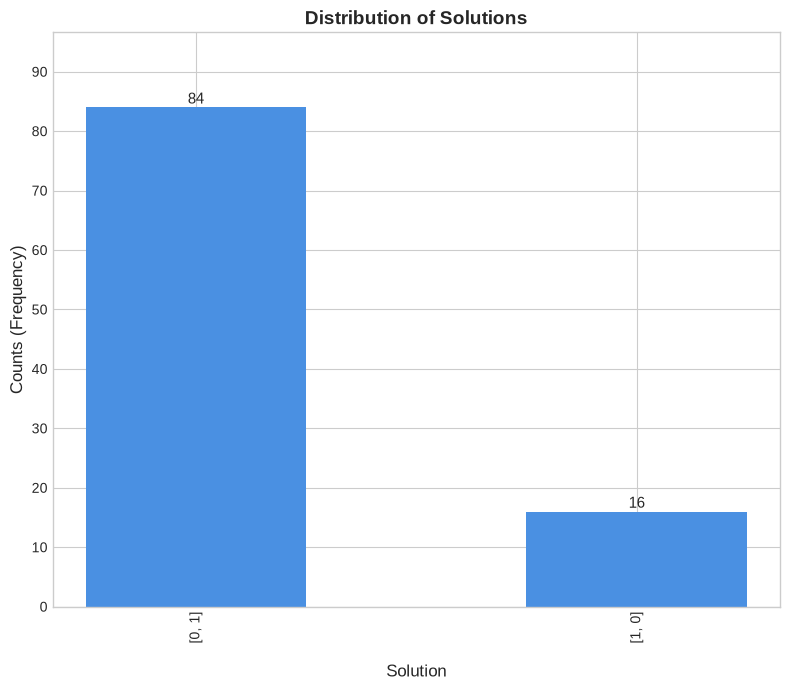
Solving Quadratic Unconstrained Binary Optimization (QUBO) Problems via Dirac-3 Integer Solver
A Quadratic Unconstrained Binary Optimization (QUBO) problem is defined by the goal of minimizing the following objective function, E, over a set of binary variables:
where the variables are binary, i.e., , where are the linear coefficients, are the quadratic coefficients, and is an offset term.
The Dirac-3 Integer Solver is specifically designed to solve problems of this nature.
To submit a QUBO problem, you provide the C and J Hamiltonians to the QuadraticModel.
The constant offset is not passed to the model directly; instead, it should be stored separately and added to the final energy value returned by the solver to get the true objective function value.
Example
Suppose we want to solve the following linear integer problem via QUBO $$ \min_{\mathbf{x}} 2𝑥_0+4𝑥_1+4𝑥_2+4𝑥_3+4𝑥_4+4𝑥_5+5𝑥_6+4𝑥_7+5𝑥_8+6𝑥_9+5𝑥_{10} \ s.t. \begin{bmatrix} 1 & 0 & 0 & 1 & 1 & 1 & 0 & 1 & 1 & 1 & 1\ 0 & 1 & 0 & 1 & 0 & 1 & 1 & 0 & 1 & 1 & 1\ 0 & 0 & 1 & 0 & 1 & 0 & 1 & 1 & 1 & 1 & 1 \end{bmatrix}\mathbf{x}=
\mathbf{x} \in {0,1 }^{11} $$
First, we rewrite this problem as an unconstrained one by adding quadratic penalties for the linear constraints. Let’s define the problem parameters.
A = np.array([[1, 0, 0, 1, 1, 1, 0, 1, 1, 1, 1],
            [0, 1, 0, 1, 0, 1, 1, 0, 1, 1, 1],
            [0, 0, 1, 0, 1, 0, 1, 1, 1, 1, 1]])
b = np.array([1, 1, 1])
c = np.array([2, 4, 4, 4, 4, 4, 5, 4, 5, 6, 5])
num_variables = A.shape[1]
Given the parameters, we can solve the problem using classical methods.
However, we can also use the eqc_models library to solve this problem using the Dirac-3 Integer solver.
# Build a Pyomo model for the constrained linear integer program
m = pyo.ConcreteModel(name="Constrained_Linear_Integer_Program")

# Define the set of variable indices
m.I = pyo.RangeSet(0, num_variables - 1)
# Define the set of constraint indices
m.J = pyo.RangeSet(0, A.shape[0] - 1)

# Define the 11 binary variables
m.x = pyo.Var(m.I, domain=pyo.Binary)

# Define the Objective Function
# The objective is the original linear expression.
m.obj = pyo.Objective(
    expr=sum(c[i] * m.x[i] for i in m.I),
    sense=pyo.minimize
)

# Define the constraints
# We define a set of constraints Ax = b directly.
def ax_constraint_rule(model, j):
    # For each row j, sum(A[j,i] * x[i]) must equal b[j]
    return sum(A[j, i] * model.x[i] for i in model.I) == b[j]

m.constraints = pyo.Constraint(m.J, rule=ax_constraint_rule)

# Solve the model
# We use a Mixed-Integer Linear Programming (MILP) solver.
solver = pyo.SolverFactory('highs')
if not solver.available(exception_flag=False):
    raise RuntimeError("HiGHS not found. Install the locked QCi environment above.")
results = solver.solve(m, tee=False)
pyo.assert_optimal_termination(results)

# Exhaustive enumeration is inexpensive for 11 dimensionless binary variables.
local_candidates = np.array(list(itertools.product([0, 1], repeat=num_variables)))
feasible_mask = np.all(local_candidates @ A.T == b, axis=1)
feasible_costs = local_candidates[feasible_mask] @ c
local_optimum = int(feasible_costs.min())
assert local_optimum == 5
np.testing.assert_allclose(pyo.value(m.obj), local_optimum)
np.testing.assert_allclose(A @ np.array([pyo.value(m.x[i]) for i in m.I]), b)

# Display the optimization results
print("\n" + "="*40)
print("-- 📊 Optimization Results --")
print(f"Solver Status: {results.solver.status}")
print(f"Termination Condition: {results.solver.termination_condition}")
print(f"Objective Value: {pyo.value(m.obj):.4f}")

print("\n-- 🏗️ Variable Values --")
solution_vector = [int(pyo.value(m.x[i])) for i in m.I]
print(f"x = {solution_vector}")
========================================
-- 📊 Optimization Results --
Solver Status: ok
Termination Condition: optimal
Objective Value: 5.0000

-- 🏗️ Variable Values --
x = [0, 0, 0, 0, 0, 0, 0, 0, 1, 0, 0]
To define the C and J matrices, we reformulate the linear problem
as follows:
where is a penalization factor that ensures the constraints are satisfied.
The term penalizes deviations from the constraints.
From this reformulation, we can derive the quadratic hamiltonian, linear hamiltonian and offset as follows:
Penalty parameter rationale
The penalty term must be large enough that any infeasible assignment is worse than the objective improvement it might gain by violating the constraint. For a binary constraint A x = b, the residual A x - b is integer-valued; the smallest nonzero violation has squared penalty at least 1. A conservative sufficient bound is rho = sum(abs(c)) + epsilon, because changing binary variables can improve the linear objective by at most sum(abs(c_i)).
Worked example: if sum(abs(c_i)) = 6 and rho = 5.9, an infeasible assignment with violation 1 can gain 6 objective units while paying only 5.9 penalty units, so it can look 0.1 units better than a feasible assignment. Choosing rho = 6 + epsilon closes that gap for this bounded binary model.
This is a sufficient bound for this model family, not a universal rule. Constraints with non-binary variables, non-integer residuals, or a larger objective range need a problem-specific penalty analysis. See Glover, Kochenberger, and Du (2019), “A Tutorial on Formulating and Using QUBO Models.”
epsilon = 1 # choose rho strictly above the sufficient penalty bound
rho = np.sum(np.abs(c)) + epsilon # penalty multiplier

# Construct the quadratic Hamiltonian J
J = rho*np.matmul(A.T,A)

# Construct the linear Hamiltonian C
C = c.copy()
C -= rho*2*(np.matmul(b.T,A))

# Construct the offset term cQ
cQ = rho*np.matmul(b.T,b)

# --- Formatted Printing ---
print("\n" + "="*60)
print("--- QUBO Formulation Parameters ---")
# Set numpy print options for better readability
np.set_printoptions(precision=2, suppress=True)

print("\nQuadratic Hamiltonian (J):\n", J)
print("\n" + "-"*60)
print("\nLinear Hamiltonian (C):\n", C)
print("\n" + "-"*60)
print(f"\nOffset Term (cQ): {cQ:.2f}")
print("\n" + "="*60)
============================================================
--- QUBO Formulation Parameters ---

Quadratic Hamiltonian (J):
 [[ 48   0   0  48  48  48   0  48  48  48  48]
 [  0  48   0  48   0  48  48   0  48  48  48]
 [  0   0  48   0  48   0  48  48  48  48  48]
 [ 48  48   0  96  48  96  48  48  96  96  96]
 [ 48   0  48  48  96  48  48  96  96  96  96]
 [ 48  48   0  96  48  96  48  48  96  96  96]
 [  0  48  48  48  48  48  96  48  96  96  96]
 [ 48   0  48  48  96  48  48  96  96  96  96]
 [ 48  48  48  96  96  96  96  96 144 144 144]
 [ 48  48  48  96  96  96  96  96 144 144 144]
 [ 48  48  48  96  96  96  96  96 144 144 144]]

------------------------------------------------------------

Linear Hamiltonian (C):
 [ -94  -92  -92 -188 -188 -188 -187 -188 -283 -282 -283]

------------------------------------------------------------

Offset Term (cQ): 144.00

============================================================
Since the QuadraticModel cannot handle the offset term directly, we will store it separately and add it to the final energy value returned by the solver to get the true objective function value.
model = QuadraticModel(C, J)
model.upper_bound = np.ones((11, )) # Set the upper bound for the variables

# Match every energy to the original objective plus squared residual penalties.
manual_energies = np.array([model.evaluate(x) + cQ for x in local_candidates])
reference_energies = local_candidates @ c + rho * np.sum((local_candidates @ A.T - b)**2, axis=1)
np.testing.assert_allclose(manual_energies, reference_energies)
local_minimizers = local_candidates[manual_energies == manual_energies.min()]
assert manual_energies.min() == local_optimum
assert np.all(local_minimizers @ A.T == b)
print(f"Validated {len(local_candidates)} QUBO energies; local optimum = {local_optimum}.")

qubo_response = None
if enable_qci_cloud:
    solver = Dirac3IntegerCloudSolver(url=api_url, api_token=api_token)
    Q = model.qubo.Q

    qubo_response = solve_without_provider_identifiers(solver, model, num_samples=10) # qubomodel

    solution = model.decode(np.array(qubo_response["results"]["solutions"][0]), "qubo")

    true_solution = model.evaluate(solution) + cQ # add the offset term to get the true objective value

    print(f"Decoded Solution (x): {solution}")
    print(f"Objective Value (E): {true_solution}")
else:
    print("Skipped QCi cloud submission; QUBO checked locally.")
QCI job completed; provider identifiers are omitted from notebook output.
Decoded Solution (x): [0 0 0 0 0 0 0 0 1 0 0]
Objective Value (E): 5
if qubo_response is not None:
    # Plot the distribution of unique solutions
    plot_solution_distribution(qubo_response)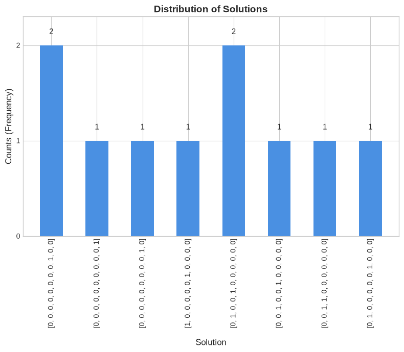
Solving the Problem in Constrained Polynomial Form
We can now define the problem using the ConstrainedPolynomialModel class, which will automatically convert the linear constraints into a penalty function and combine them with the original objective. This approach avoids the need to manually construct a QUBO matrix.
To use this model, we provide the objective and constraints separately:
coefficientsandindices: These define the original linear objective function, . The coefficients variable holds the vector c of costs, while indices specifies the variable for each corresponding coefficient.lhsandrhs: These define the linear equality constraints, . Thelhsvariable is the left-hand-side matrixA, andrhsis the right-hand-side vectorb.
coefficients = c
num_vars = 11
indices = [[0, i + 1] for i in range(num_vars)]

lhs = A
rhs = b

# ConstrainedPolynomialModel wraps the QUBO with explicit constraints.
constraint_model = ScalarConstrainedPolynomialModel(coefficients, indices, lhs, rhs)
constraint_model.upper_bound = np.ones(num_vars, ) # Set the upper bound for the variables
# Set the penalty multiplier for the constraints
# This is a crucial step to ensure the constraints are satisfied in the optimization process.
constraint_model.penalty_multiplier = np.sum(np.abs(c)) + 1  # Set the penalty multiplier
print(constraint_model.offset) # Offset term generated by the model

# Check the independent constrained representation, including its offset.
constrained_energies = np.asarray([
    constraint_model.evaluate(x) for x in local_candidates
]).reshape(-1) + constraint_model.offset * constraint_model.penalty_multiplier
np.testing.assert_allclose(constrained_energies, reference_energies)
for candidate in local_candidates:
    np.testing.assert_allclose(constraint_model.evaluateObjective(candidate), c @ candidate)
    np.testing.assert_allclose(
        constraint_model.evaluatePenalties(candidate, include_offset=True),
        np.sum((A @ candidate - b)**2),
    )
print("Validated constrained objective, penalties, and offset for all binary assignments.")

constrained_response = None
if enable_qci_cloud:
    solver = Dirac3IntegerCloudSolver(url=api_url, api_token=api_token)
    constrained_response = solve_without_provider_identifiers(
        solver,
        constraint_model,
        num_samples=10,
    )

else:
    print("Skipped QCi cloud submission; constrained model checked locally.")
3
QCI job completed; provider identifiers are omitted from notebook output.
if constrained_response is not None:
    # plot the distribution of unique solutions
    plot_solution_distribution(constrained_response)

    # Extract the best solution and its objective value
    best_solution = constrained_response["results"]["solutions"][0]
    best_objective_value = constrained_response["results"]["energies"][0] + constraint_model.offset * constraint_model.penalty_multiplier
    # Add the offset term to get the true objective value

    print(f"Best Solution: {best_solution}")
    print(f"Best Objective Value: {best_objective_value}")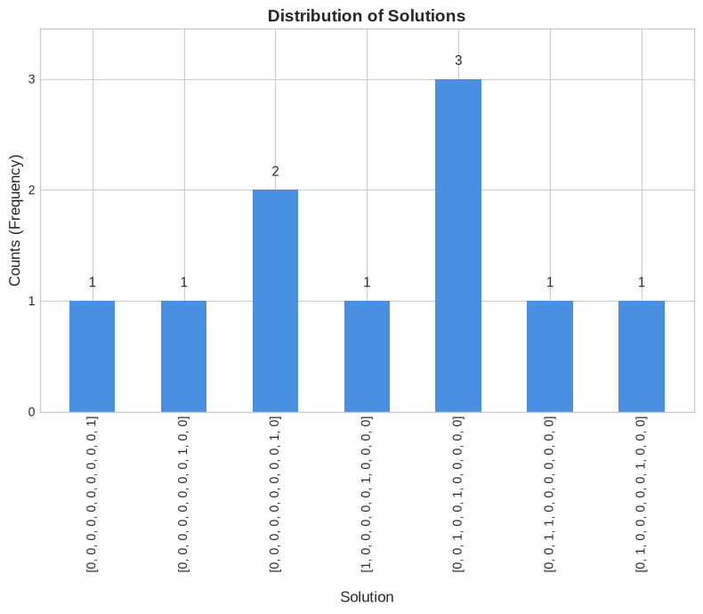
Best Solution: [0, 0, 0, 0, 0, 0, 0, 0, 0, 0, 1]
Best Objective Value: 5
Practice checkpoints
Use these checkpoints during the workshop to test the main ideas before moving on.
# =============================================================================
# EXERCISE 1: Adjust the sum constraint
# =============================================================================
# Change the sum constraint in the small QCi example and predict how the feasible solution set changes before submitting or enumerating the model.
#
# Hint: For credential-free validation, enumerate a tiny version locally.
#
# Your code here:
# =============================================================================
Notebook Cell
# SOLUTION (hidden in workshop version):
# Enumerate a small sum-constrained candidate set locally.
import itertools

target_sum = 2
candidates = [
    bits
    for bits in itertools.product([0, 1], repeat=3)
    if sum(bits) == target_sum
]
print({"target_sum": target_sum, "feasible_candidates": candidates})
{'target_sum': 2, 'feasible_candidates': [(0, 1, 1), (1, 0, 1), (1, 1, 0)]}
# =============================================================================
# EXERCISE 2: Validate a small QUBO locally
# =============================================================================
# Before submitting a two-variable model, enumerate all binary assignments and compute the energy by hand or with a short helper.
#
# Hint: There are only four assignments.
#
# Your code here:
# =============================================================================
Notebook Cell
# SOLUTION (hidden in workshop version):
# Validate a two-variable QUBO before cloud submission.
import itertools

def small_qubo_energy(bits):
    x0, x1 = bits
    return -x0 - x1 + 2 * x0 * x1

energies = {
    bits: small_qubo_energy(bits)
    for bits in itertools.product([0, 1], repeat=2)
}
print(min(energies.items(), key=lambda item: item[1]))
((0, 1), -1)
# =============================================================================
# EXERCISE 3: Plan for missing credentials
# =============================================================================
# Write down which cells can run without QCi credentials and which must be skipped. Add a fallback analysis that still checks model construction.
#
# Hint: Separate model-building validation from cloud submission.
#
# Your code here:
# =============================================================================
Notebook Cell
# SOLUTION (hidden in workshop version):
# Separate credential-free model checks from cloud execution.
credential_free_checks = [
    "imports",
    "model construction",
    "local objective evaluation",
]
requires_qci_token = ["submit job", "poll job", "download cloud result"]
print({"local": credential_free_checks, "cloud": requires_qci_token})
{'local': ['imports', 'model construction', 'local objective evaluation'], 'cloud': ['submit job', 'poll job', 'download cloud result']}
Summary
In this notebook we:
Introduced QCi’s entropy-computing workflow and the Dirac-3 solver interface for constrained optimization.
Built constrained quadratic and polynomial model representations from linear objective and constraint data.
Submitted models to QCi solvers when credentials are available and decoded the returned solution vectors and energies.
Compared manual QUBO offset handling with the constrained polynomial model abstraction.
Learning objectives met: You practiced describing the Dirac modeling workflow, constructing constrained models, decoding solver responses, and comparing explicit QUBO penalties with higher-level constraint handling.
Next steps: This is the final Python notebook in the current sequence; use the benchmarking notebook to design fair comparisons when applying QCi models to your own optimization instances.
Further reading:
References
Nguyen, L., et al. (2024). Entropy Computing: A Paradigm for Optimization in an Open Quantum System. arXiv preprint arXiv:2407.04512. Retrieved from https://
arxiv .org /abs /2407 .04512 Nguyen, L., et al. (2025). Entropy computing, a paradigm for optimization in open photonic systems. Communications Physics, 8, Article 411. Retrieved from https://
www .nature .com /articles /s42005 -025 -02324-6 Quantum Computing Inc. (2024). Dirac-3 User Guide. Retrieved from https://
quantumcomputinginc .com /learn /support /user -guides /dirac -3 -user -guide
David E. Bernal Neira — Davidson School of Chemical Engineering, Purdue University
Albert Lee — Davidson School of Chemical Engineering, Purdue University; Graduate Research Assistant
Acknowledgments
This notebook was developed by: