
Setup
Google Colab
Click the badge above to open this notebook in Colab. The notebook installs or activates dependencies in the setup cells below.
Local installation
Run the following from the repository root before opening this notebook locally:
uv sync --locked --group docs --group mathprog
uv run --locked --group docs --group mathprog idaes get-extensions --release 3.4.2 --to .nbverify/mathprog-solvers
export PATH="$PWD/.nbverify/mathprog-solvers:$PATH"
make verify-mathprog-python-local
Install GLPK separately as described below; the Ubuntu command also installs the IDAES runtime libraries. CBC, IPOPT, BONMIN, and Couenne come from the IDAES solver bundle. All five solvers are required: a missing executable or failed solve stops verification. The local target executes the complete notebook under warnings-as-errors and writes fresh results to .nbverify/; no credentials are needed.
See local-setup.md for the full local workflow, including optional commercial solver licences.
GLPK (required for ILP sections):
macOS:
brew install glpkUbuntu/Debian:
sudo apt-get install glpk-utils libgfortran5 libgomp1 liblapack3 libblas3Windows: download from http://
winglpk .sourceforge .net/
Learning objectives
By the end of this notebook you will be able to:
Formulate linear, integer, convex nonlinear, and nonconvex nonlinear programs from a word problem.
Implement the same optimization model family in Pyomo with continuous and integer decision variables.
Select appropriate LP, MILP, NLP, and MINLP solvers and interpret their reported solutions.
Explain how integrality and nonconvexity change the difficulty and reliability of optimization workflows.
Prerequisites
Mathematical background: Basic algebra, inequalities, objective functions, and familiarity with continuous and integer variables.
Prior notebooks: None; this is the first Python notebook in the sequence.
Accounts required: None. Every solver this notebook uses is open source.
Python version: Python 3.9+ with the Pyomo stack used by this repository.
Introduction to Mathematical Programming
Modeling
The solution of optimization problems requires the development of a mathematical model. Here we will model an example given in the lecture and see how an integer program can be solved practically. This example will use as modeling language Pyomo, an open-source Python package, which provides a flexible access to different solvers and a general modeling framework for linear and nonlinear integer programs. The examples solved here will make use of open-source solvers GLPK and CLP/CBC for linear and mixed-integer linear programming, IPOPT for interior point (non)linear programming, BONMIN for convex integer nonlinear programming and COUENNE for nonconvex (global) integer nonlinear programming.
Notebook Cell
# If using this on Google Colab, we need to install the packages
try:
  import google.colab
  IN_COLAB = True
except:
  IN_COLAB = False

# Let's start with Pyomo
if IN_COLAB:
    !pip install -q pyomo idaes-pse matplotlib numpy scipy
# Import the Pyomo library, which can be installed via pip, conda, or from GitHub: https://github.com/Pyomo/pyomo
import pyomo.environ as pyo
# Import Matplotlib to generate plots
import matplotlib.pyplot as plt
# Import numpy and scipy for certain numerical calculations below
import numpy as np
from scipy.special import gamma
import math
import os
Problem statement
Suppose there is a company that produces two different products, A and B, which can be sold at different values, and per unit, respectively. The company has a single machine with electricity use capped at 17 kW/day. Producing each unit of A and B consumes and , respectively. Besides, the company can only produce at most 2 more units of B than A per day.
Linear Programming
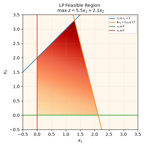
This is a valid model, but it would be easier to solve if we had a mathematical representation. Assuming the units produced of A are and of B are we have
# Generate the feasible region plot of this problem

# Define meshgrid for feasible region
d = np.linspace(-0.5,3.5,300)
x1,x2 = np.meshgrid(d,d)

# Define the lines for the constraints
x = np.linspace(x1.min(), x1.max(), 2000)
# x2 <= x1 + 2
x21 = x + 2
# 8*x1 + 2*x2 <= 17
x22 = (17-8*x)/2.0
# Objective: max 5.5*x1 + 2.1*x2
# generate heatmap from objective function
objective_heatmap = np.fromfunction(lambda i, j:5.5 * i + 2.1 * j,(300,300), dtype=float)

# Plot feasible region
fig, ax = plt.subplots()
feas_reg = ax.imshow( (
    (x1>=0) &           # Bound 1
    (x2>=0) &           # Bound 2
    (x2 <= x1 + 2) &    # Constraint 1
    (8*x1 + 2*x2 <= 17) # Constraint 2
    ).astype(int)
    * objective_heatmap, # objective function
                extent=(x1.min(),x1.max(),x2.min(),x2.max()),origin="lower", cmap="OrRd", alpha = 1)

# Make plots of constraints
ax.plot(x, x21, label=r'$x_2 \leq x_1 + 2$')
ax.plot(x, x22, label=r'$8x_1 + 2x_2 \leq 17$')

# Nonnegativitivy constraints
plt.plot(x, np.zeros_like(x), label=r'$x_2 \geq 0$')
plt.plot(np.zeros_like(x), x, label=r'$x_1 \geq 0$')

# plot formatting
plt.title("LP Feasible Region \n max $z = 5.5x_{1} + 2.1x_{2}$",fontsize=10,y=1)
plt.xlim(x1.min(),x1.max())
plt.ylim(x2.min(),x2.max())
plt.legend(loc='upper right', prop={'size': 6})
plt.xlabel(r'$x_1$')
plt.ylabel(r'$x_2$')
plt.grid(alpha=0.2)
# Define the model
model = pyo.ConcreteModel(name='Simple example LP')
# Define the variables
model.x = pyo.Var([1,2], domain=pyo.NonNegativeReals)
# Define the objective function
def _obj(m):
    return 5.5*m.x[1] + 2.1*m.x[2]

model.obj = pyo.Objective(rule = _obj, sense=pyo.maximize)
# Define the constraints
def _constraint1(m):
    return m.x[2] <= m.x[1] + 2

def _constraint2(m):
    return 8*m.x[1] + 2*m.x[2] <= 17

model.Constraint1 = pyo.Constraint(rule = _constraint1)

model.Constraint2 = pyo.Constraint(rule = _constraint2)
# Print the model
model.pprint()
1 Var Declarations
x : Size=2, Index={1, 2}
Key : Lower : Value : Upper : Fixed : Stale : Domain
1 : 0 : None : None : False : True : NonNegativeReals
2 : 0 : None : None : False : True : NonNegativeReals
1 Objective Declarations
obj : Size=1, Index=None, Active=True
Key : Active : Sense : Expression
None : True : maximize : 5.5*x[1] + 2.1*x[2]
2 Constraint Declarations
Constraint1 : Size=1, Index=None, Active=True
Key : Lower : Body : Upper : Active
None : -Inf : x[2] - (x[1] + 2) : 0.0 : True
Constraint2 : Size=1, Index=None, Active=True
Key : Lower : Body : Upper : Active
None : -Inf : 8*x[1] + 2*x[2] : 17.0 : True
4 Declarations: x obj Constraint1 Constraint2
Notebook Cell
# Let's install the LP/MIP solvers GLPK and CBC
if IN_COLAB:
    !apt-get install -y -qq glpk-utils
    !apt-get install -y -qq coinor-cbc
# Define the solvers GLPK and CBC
if IN_COLAB:
    opt_glpk = pyo.SolverFactory('glpk', executable='/usr/bin/glpsol')
    opt_cbc = pyo.SolverFactory('cbc', executable='/usr/bin/cbc')
else:
    opt_glpk = pyo.SolverFactory('glpk')
    opt_cbc = pyo.SolverFactory('cbc')

for solver_name, solver in [('GLPK', opt_glpk), ('CBC', opt_cbc)]:
    if not solver.available(exception_flag=False):
        raise RuntimeError(f"{solver_name} not found. Run the GLPK/CBC install cell above.")
    print(f"{solver_name}: OK")
# Here we could use another solver, e.g. gurobi or cplex
# opt_gurobi = pyo.SolverFactory('gurobi')
GLPK: OK
CBC: OK
# Each solve checks termination and feasibility, and compares the objective
# with the tutorial's known optimum when supplied (14.08 for this LP).
# A failed check stops execution. BONMIN's nonconvex example omits the
# objective check because it cannot certify a global optimum.
def check_solution(model, results, expected_objective=None):
    """Check termination, feasibility, and the tutorial's known objective.

    Absolute tolerance 1e-6 in each model expression's units accommodates
    solver feasibility slack without hiding a wrong solution.
    Omit expected_objective for BONMIN on the nonconvex model, where it
    cannot certify a global optimum.
    """
    pyo.assert_optimal_termination(results)
    tolerance = 1e-6
    for variable in model.component_data_objects(pyo.Var, active=True):
        value = pyo.value(variable)
        assert math.isfinite(value), "Non-finite decision variable"
        if variable.lb is not None:
            assert value >= variable.lb - tolerance, "Variable below its lower bound"
        if variable.ub is not None:
            assert value <= variable.ub + tolerance, "Variable above its upper bound"
        if variable.is_integer():
            assert abs(value - round(value)) <= tolerance, "Non-integer decision"
    for constraint in model.component_data_objects(pyo.Constraint, active=True):
        value = pyo.value(constraint.body)
        assert math.isfinite(value), "Non-finite constraint residual"
        if constraint.has_lb():
            assert value >= pyo.value(constraint.lower) - tolerance, "Constraint lower bound violated"
        if constraint.has_ub():
            assert value <= pyo.value(constraint.upper) + tolerance, "Constraint upper bound violated"
    if expected_objective is not None:
        assert math.isclose(pyo.value(model.obj), expected_objective,
                            rel_tol=0, abs_tol=tolerance), "Unexpected objective"

# Here we solve the optimization problem, the option tee=True prints the solver output
result_obj = opt_glpk.solve(model, tee=True)
check_solution(model, result_obj, expected_objective=14.08)
GLPSOL--GLPK LP/MIP Solver 5.0
Parameter(s) specified in the command line:
 --write <TEMPORARY_PATH> --wglp <TEMPORARY_PATH> --cpxlp
 <TEMPORARY_PATH>
Reading problem data from '<TEMPORARY_PATH>'...
2 rows, 2 columns, 4 non-zeros
23 lines were read
Writing problem data to '<TEMPORARY_PATH>'...
15 lines were written
GLPK Simplex Optimizer 5.0
2 rows, 2 columns, 4 non-zeros
Preprocessing...
2 rows, 2 columns, 4 non-zeros
Scaling...
 A: min|aij| =  1.000e+00  max|aij| =  8.000e+00  ratio =  8.000e+00
Problem data seem to be well scaled
Constructing initial basis...
Size of triangular part is 2
*     0: obj =  -0.000000000e+00 inf =   0.000e+00 (2)
*     2: obj =   1.408000000e+01 inf =   0.000e+00 (0)
OPTIMAL LP SOLUTION FOUND
Time used:   0.0 secs
Memory used: 0.0 Mb (39693 bytes)
Writing basic solution to '<TEMPORARY_PATH>'...
13 lines were written
# Display solution of the problem
model.display()
Model Simple example LP
Variables:
x : Size=2, Index={1, 2}
Key : Lower : Value : Upper : Fixed : Stale : Domain
1 : 0 : 1.3 : None : False : False : NonNegativeReals
2 : 0 : 3.3 : None : False : False : NonNegativeReals
Objectives:
obj : Size=1, Index=None, Active=True
Key : Active : Value
None : True : 14.08
Constraints:
Constraint1 : Size=1
Key : Lower : Body : Upper
None : None : 0.0 : 0.0
Constraint2 : Size=1
Key : Lower : Body : Upper
None : None : 17.0 : 17.0
# Optimal solution LP
ax.scatter(1.3,3.3,color='r', label='optimal solution LP')
ax.get_legend().remove()
ax.legend(bbox_to_anchor=(1.05, 1), loc=2, borderaxespad=0.)
fig.canvas.draw()
fig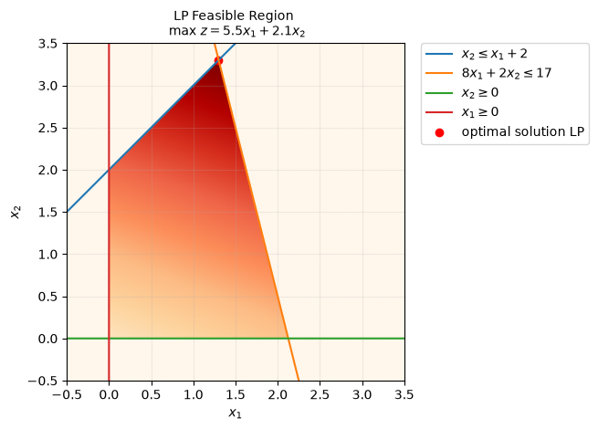
We observe that the optimal solution of this problem is , , leading to a profit of 14.08.
# We obtain the same solution with CBC
result_obj = opt_cbc.solve(model, tee=False)
check_solution(model, result_obj, expected_objective=14.08)
model.display()
Model Simple example LP

  Variables:
    x : Size=2, Index={1, 2}
        Key : Lower : Value : Upper : Fixed : Stale : Domain
          1 :     0 :   1.3 :  None : False : False : NonNegativeReals
          2 :     0 :   3.3 :  None : False : False : NonNegativeReals

  Objectives:
    obj : Size=1, Index=None, Active=True
        Key  : Active : Value
        None :   True : 14.08

  Constraints:
    Constraint1 : Size=1
        Key  : Lower : Body : Upper
        None :  None :  0.0 :   0.0
    Constraint2 : Size=1
        Key  : Lower : Body : Upper
        None :  None : 17.0 :  17.0
The solvers GLPK and CLP implement the simplex method (with many improvements) by default, but we can also use the interior-point solver IPOPT. IPOPT can solve both linear and nonlinear problems.
Notebook Cell
# Install IDAES solver extensions and configure IPOPT
if IN_COLAB:
    !pip install idaes-pse==2.12.0
    !idaes get-extensions --to ./solvers
    os.environ['PATH'] += ':solvers'
    for solver_name in ['ipopt', 'bonmin', 'couenne']:
        solver = pyo.SolverFactory(solver_name, executable=f'/content/solvers/{solver_name}')
        if not solver.available(exception_flag=False):
            raise RuntimeError(f"IDAES extension install did not provide {solver_name}. Check the install output above.")
        print(f"{solver_name}: OK")
    opt_ipopt = pyo.SolverFactory('ipopt', executable='/content/solvers/ipopt')
else:
    opt_ipopt = pyo.SolverFactory('ipopt')
if not opt_ipopt.available(exception_flag=False):
    raise RuntimeError("IPOPT not found. Run the IDAES solver setup cell near the top of this notebook.")
# Here we solve the optimization problem, the option tee=True prints the solver output
result_obj_ipopt = opt_ipopt.solve(model, tee=True)
check_solution(model, result_obj_ipopt, expected_objective=14.08)
model.display()
Ipopt 3.13.2:

******************************************************************************
This program contains Ipopt, a library for large-scale nonlinear optimization.
 Ipopt is released as open source code under the Eclipse Public License (EPL).
         For more information visit http://projects.coin-or.org/Ipopt

This version of Ipopt was compiled from source code available at
    https://github.com/IDAES/Ipopt as part of the Institute for the Design of
    Advanced Energy Systems Process Systems Engineering Framework (IDAES PSE
    Framework) Copyright (c) 2018-2019. See https://github.com/IDAES/idaes-pse.

This version of Ipopt was compiled using HSL, a collection of Fortran codes
    for large-scale scientific computation.  All technical papers, sales and
    publicity material resulting from use of the HSL codes within IPOPT must
    contain the following acknowledgement:
        HSL, a collection of Fortran codes for large-scale scientific
        computation. See http://www.hsl.rl.ac.uk.
******************************************************************************

This is Ipopt version 3.13.2, running with linear solver ma27.

Number of nonzeros in equality constraint Jacobian...:        0
Number of nonzeros in inequality constraint Jacobian.:        4
Number of nonzeros in Lagrangian Hessian.............:        0

Total number of variables............................:        2
                     variables with only lower bounds:        2
                variables with lower and upper bounds:        0
                     variables with only upper bounds:        0
Total number of equality constraints.................:        0
Total number of inequality constraints...............:        2
        inequality constraints with only lower bounds:        0
   inequality constraints with lower and upper bounds:        0
        inequality constraints with only upper bounds:        2

iter    objective    inf_pr   inf_du lg(mu)  ||d||  lg(rg) alpha_du alpha_pr  ls
   0 -1.4080000e+01 0.00e+00 1.09e-01  -1.0 0.00e+00    -  0.00e+00 0.00e+00   0
   1 -1.3912219e+01 0.00e+00 1.00e-06  -1.0 1.00e-01    -  1.00e+00 1.00e+00h  1
   2 -1.4069173e+01 0.00e+00 1.12e-03  -2.5 1.33e-01    -  9.84e-01 1.00e+00f  1
   3 -1.4079704e+01 0.00e+00 1.50e-09  -3.8 1.06e-02    -  1.00e+00 1.00e+00f  1
   4 -1.4079996e+01 0.00e+00 1.84e-11  -5.7 2.45e-04    -  1.00e+00 1.00e+00f  1
   5 -1.4080000e+01 0.00e+00 2.57e-14  -8.6 3.18e-06    -  1.00e+00 1.00e+00f  1

Number of Iterations....: 5

                                   (scaled)                 (unscaled)
Objective...............:  -1.4080000135787204e+01   -1.4080000135787204e+01
Dual infeasibility......:   2.5678265217212132e-14    2.5678265217212132e-14
Constraint violation....:   0.0000000000000000e+00    0.0000000000000000e+00
Complementarity.........:   2.5064622693731291e-09    2.5064622693731291e-09
Overall NLP error.......:   2.5064622693731291e-09    2.5064622693731291e-09


Number of objective function evaluations             = 6
Number of objective gradient evaluations             = 6
Number of equality constraint evaluations            = 0
Number of inequality constraint evaluations          = 6
Number of equality constraint Jacobian evaluations   = 0
Number of inequality constraint Jacobian evaluations = 6
Number of Lagrangian Hessian evaluations             = 5
Total CPU secs in IPOPT (w/o function evaluations)   =      0.001
Total CPU secs in NLP function evaluations           =      0.000

EXIT: Optimal Solution Found.
Model Simple example LP

  Variables:
    x : Size=2, Index={1, 2}
        Key : Lower : Value              : Upper : Fixed : Stale : Domain
          1 :     0 : 1.3000000135344933 :  None : False : False : NonNegativeReals
          2 :     0 : 3.3000000292130904 :  None : False : False : NonNegativeReals

  Objectives:
    obj : Size=1, Index=None, Active=True
        Key  : Active : Value
        None :   True : 14.080000135787204

  Constraints:
    Constraint1 : Size=1
        Key  : Lower : Body                  : Upper
        None :  None : 1.567859708728747e-08 :   0.0
    Constraint2 : Size=1
        Key  : Lower : Body              : Upper
        None :  None : 17.00000016670213 :  17.0
We obtain the same result as previously, but notice that the interior point method reports some solution subject to certain tolerance, given by its convergence properties when it can get infinitesimally close (but not directly at) the boundary of the feasible region.
From Linear Programming to Integer Programming
The LP above allows fractional decisions, which is useful for production rates but not for yes/no or count decisions. When the variables must be integers, the feasible region becomes a set of discrete points rather than a filled polygon. Solvers such as GLPK and CBC handle this by solving LP relaxations inside a branch-and-bound search. This usually makes the model harder, but it also lets the formulation represent decisions such as building 0, 1, or 2 units.
Integer Programming
Now let’s consider that only integer units of each product can be produced, namely
# Define grid for integer points
x1_int, x2_int = np.meshgrid(range(math.ceil(x1.max())), range(math.ceil(x2.max())))
idx = ((x1_int>=0) & (x2_int <= x1_int + 2) & (8*x1_int + 2*x2_int <= 17) & (x2_int>=0))
x1_int, x2_int = x1_int[idx], x2_int[idx]
ax.scatter(x1_int,x2_int,color='k', label='integer points')

# Plotting optimal solution IP
# plt.title("LP Feasible Region \n max $z = 5.5x_{1} + 2.1x_{2}$",fontsize=10,y=1)
ax.set_title("ILP Feasible Region \n max $z = 5.5x_{1} + 2.1x_{2}$")
ax.get_legend().remove()
ax.legend(bbox_to_anchor=(1.05, 1), loc=2, borderaxespad=0.)
fig.canvas.draw()
fig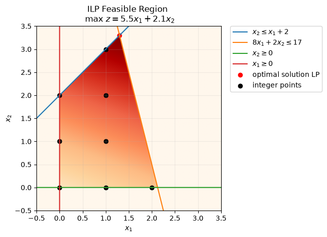
# Define the integer model
model_ilp = pyo.ConcreteModel(name='Simple example IP, 47-779 QuIP')
#Define the variables
model_ilp.x = pyo.Var([1,2], domain=pyo.Integers)
# Define the objective function
model_ilp.obj = pyo.Objective(rule = _obj, sense=pyo.maximize)
# Define the constraints
model_ilp.Constraint1 = pyo.Constraint(rule = _constraint1)

model_ilp.Constraint2 = pyo.Constraint(rule = _constraint2)
# Print the model
model_ilp.pprint()
1 Var Declarations
x : Size=2, Index={1, 2}
Key : Lower : Value : Upper : Fixed : Stale : Domain
1 : None : None : None : False : True : Integers
2 : None : None : None : False : True : Integers
1 Objective Declarations
obj : Size=1, Index=None, Active=True
Key : Active : Sense : Expression
None : True : maximize : 5.5*x[1] + 2.1*x[2]
2 Constraint Declarations
Constraint1 : Size=1, Index=None, Active=True
Key : Lower : Body : Upper : Active
None : -Inf : x[2] - (x[1] + 2) : 0.0 : True
Constraint2 : Size=1, Index=None, Active=True
Key : Lower : Body : Upper : Active
None : -Inf : 8*x[1] + 2*x[2] : 17.0 : True
4 Declarations: x obj Constraint1 Constraint2
# Here we solve the optimization problem, the option tee=True prints the solver output
result_obj_ilp = opt_cbc.solve(model_ilp, tee=False)
check_solution(model_ilp, result_obj_ilp, expected_objective=11.8)
model_ilp.display()Model 'Simple example IP, 47-779 QuIP'
Variables:
x : Size=2, Index={1, 2}
Key : Lower : Value : Upper : Fixed : Stale : Domain
1 : None : 1.0 : None : False : False : Integers
2 : None : 3.0 : None : False : False : Integers
Objectives:
obj : Size=1, Index=None, Active=True
Key : Active : Value
None : True : 11.8
Constraints:
Constraint1 : Size=1
Key : Lower : Body : Upper
None : None : 0.0 : 0.0
Constraint2 : Size=1
Key : Lower : Body : Upper
None : None : 14.0 : 17.0
# Optimal solution ILP
ax.scatter(1,3,color='c', label='optimal solution ILP')
ax.get_legend().remove()
ax.legend(bbox_to_anchor=(1.05, 1), loc=2, borderaxespad=0.)
fig.canvas.draw()
fig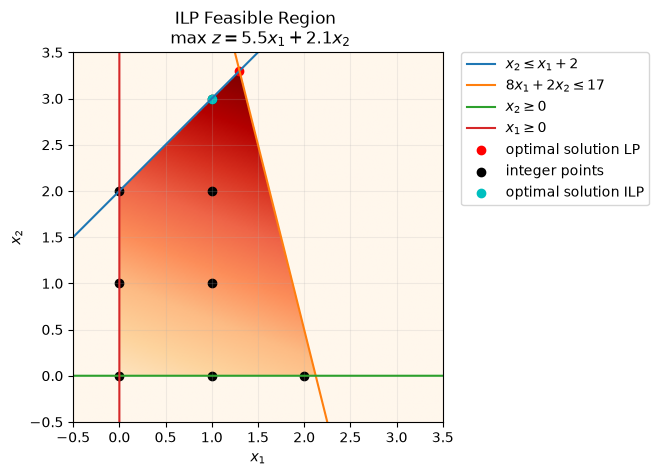
Here the solution becomes with an objective of 11.8.
Enumeration
Enumeration is practical for this small problem: the plot shows only 8 feasible integer points. If both nonnegative integer variables instead had upper bounds of 4, there would be candidate pairs before checking feasibility. With more variables, enumeration quickly becomes impractical. For binary variables (integer variables can be encoded in binary), the number of possible assignments is .
In many other applications, the possible solutions come from permutations of the integer variables (e.g. assignment problems), which grow as with the size of the input.
This combinatorial growth makes exhaustive enumeration impractical very quickly.
fig2, ax2 = plt.subplots()
n = np.arange(1,100,1)
ax2.plot(n,np.exp(n*np.log(2)), label=r'$2^n$')
ax2.plot(n,gamma(n), label=r'$n!$')

ax2.plot(n,3.154E16*np.ones_like(n), 'g--', label=r'ns in a year')
ax2.plot(n,4.3E26*np.ones_like(n), 'k--', label=r'age of the universe in ns')
ax2.plot(n,6E79*np.ones_like(n), 'r--', label=r'atoms in the universe')
plt.yscale('log')

plt.legend()
plt.xlabel(r'$n$')
plt.ylabel('Possible solutions')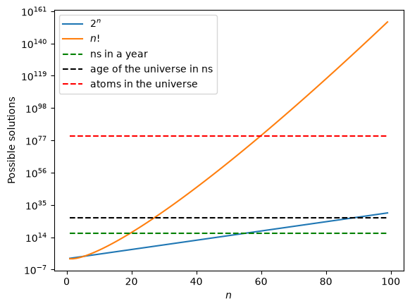
From Integer Linear Programming to Integer Nonlinear Programming
Integer variables can also appear inside nonlinear relationships. The next model keeps the same integer decision logic but adds a convex nonlinear constraint, so the feasible points are still discrete while the relaxation is curved. This changes both the geometry and the solver requirements: MILP solvers are no longer enough, and nonlinear branch-and-bound methods need problem-specific assumptions to give reliable answers.
Integer convex nonlinear programming
The following constraint “the production of B minus 1 squared can only be smaller than 2 minus the production of A” can be incorporated in the following convex integer nonlinear program
# Define grid for integer points
# Remove the previous heatmap if this cell is re-run out of order.
try:
    feas_reg.remove()
except (ValueError, AttributeError, NameError):
    pass  # already removed or not yet created
feas_reg = ax.imshow( (
    (x1>=0) &           # Bound 1
    (x2>=0) &           # Bound 2
    (x2 <= x1 + 2) &    # Constraint 1
    (8*x1 + 2*x2 <= 17) & # Constraint 2
    ((x2-1)**2 <= 2-x1) # Nonlinear constraint
    ).astype(int)
    * objective_heatmap, # objective function,
                extent=(x1.min(),x1.max(),x2.min(),x2.max()),origin="lower", cmap="OrRd", alpha = .8)


x1nl = 2- (x - 1)**2
# Nonlinear constraint
nl_const = ax.plot(x1nl, x, label=r'$(x_2-1)^2 \leq 2-x_1$')

# Plotting optimal solution INLP
ax.set_title("INLP Feasible Region \n max $z = 5.5x_{1} + 2.1x_{2}$")
ax.get_legend().remove()
ax.legend(bbox_to_anchor=(1.05, 1), loc=2, borderaxespad=0.)
fig.canvas.draw()
fig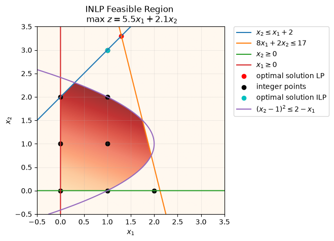
# Define the integer model
model_cinlp = pyo.ConcreteModel(name='Simple example convex INLP, 47-779 QuIP')
#Define the variables
model_cinlp.x = pyo.Var([1,2], domain=pyo.Integers)
# Define the objective function
model_cinlp.obj = pyo.Objective(rule = _obj, sense=pyo.maximize)
# Define the constraints
model_cinlp.Constraint1 = pyo.Constraint(rule = _constraint1)

model_cinlp.Constraint2 = pyo.Constraint(rule = _constraint2)

model_cinlp.Constraint3 = pyo.Constraint(expr = (model_cinlp.x[2]-1)**2 <= 2 - model_cinlp.x[1])


# Print the model
model_cinlp.pprint()
1 Var Declarations
x : Size=2, Index={1, 2}
Key : Lower : Value : Upper : Fixed : Stale : Domain
1 : None : None : None : False : True : Integers
2 : None : None : None : False : True : Integers
1 Objective Declarations
obj : Size=1, Index=None, Active=True
Key : Active : Sense : Expression
None : True : maximize : 5.5*x[1] + 2.1*x[2]
3 Constraint Declarations
Constraint1 : Size=1, Index=None, Active=True
Key : Lower : Body : Upper : Active
None : -Inf : x[2] - (x[1] + 2) : 0.0 : True
Constraint2 : Size=1, Index=None, Active=True
Key : Lower : Body : Upper : Active
None : -Inf : 8*x[1] + 2*x[2] : 17.0 : True
Constraint3 : Size=1, Index=None, Active=True
Key : Lower : Body : Upper : Active
None : -Inf : (x[2] - 1)**2 - (2 - x[1]) : 0.0 : True
5 Declarations: x obj Constraint1 Constraint2 Constraint3
# Define the solver BONMIN
if IN_COLAB:
    opt_bonmin = pyo.SolverFactory('bonmin', executable='/content/solvers/bonmin')
else:
    opt_bonmin = pyo.SolverFactory('bonmin')
if not opt_bonmin.available(exception_flag=False):
    raise RuntimeError("BONMIN not found. Run the IDAES solver setup cell near the top of this notebook.")
# Here we solve the optimization problem, the option tee=True prints the solver output
result_obj_cinlp = opt_bonmin.solve(model_cinlp, tee=False)
check_solution(model_cinlp, result_obj_cinlp, expected_objective=9.7)
model_cinlp.display()
Model 'Simple example convex INLP, 47-779 QuIP'

  Variables:
    x : Size=2, Index={1, 2}
        Key : Lower : Value : Upper : Fixed : Stale : Domain
          1 :  None :   1.0 :  None : False : False : Integers
          2 :  None :   2.0 :  None : False : False : Integers

  Objectives:
    obj : Size=1, Index=None, Active=True
        Key  : Active : Value
        None :   True :   9.7

  Constraints:
    Constraint1 : Size=1
        Key  : Lower : Body : Upper
        None :  None : -1.0 :   0.0
    Constraint2 : Size=1
        Key  : Lower : Body : Upper
        None :  None : 12.0 :  17.0
    Constraint3 : Size=1
        Key  : Lower : Body : Upper
        None :  None :  0.0 :   0.0
ax.scatter(1,2,color='m', label='optimal solution convex INLP')
ax.get_legend().remove()
ax.legend(bbox_to_anchor=(1.05, 1), loc=2, borderaxespad=0.)
fig.canvas.draw()
fig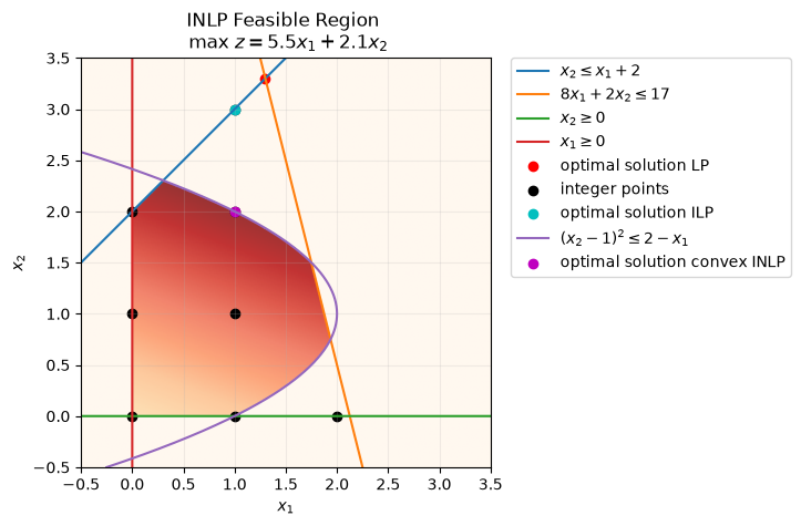
In this case the optimal solution becomes with an objective of 9.7.
Integer non-convex programming
The last constraint “the production of B minus 1 squared can only be greater than the production of A plus one half” can be incorporated in the following convex integer nonlinear program
# Define grid for integer points
# Remove the previous heatmap if this cell is re-run out of order.
try:
    feas_reg.remove()
except (ValueError, AttributeError, NameError):
    pass  # already removed or not yet created
feas_reg = ax.imshow( (
    (x1>=0) &           # Bound 1
    (x2>=0) &           # Bound 2
    (x2 <= x1 + 2) &    # Constraint 1
    (8*x1 + 2*x2 <= 17) & # Constraint 2
    ((x2-1)**2 <= 2-x1) & # Nonlinear constraint 1
    ((x2-1)**2 >= x1+0.5) # Nonlinear constraint 2
    ).astype(int)
    * objective_heatmap,  # objective function,
                extent=(x1.min(),x1.max(),x2.min(),x2.max()),origin="lower", cmap="OrRd", alpha = .8)


x1nl = -1/2 + (x - 1)**2
# Nonlinear constraint
nl_const = ax.plot(x1nl, x, label=r'$(x_2-1)^2 \geq x_1 + 1/2$')

ax.get_legend().remove()
ax.legend(bbox_to_anchor=(1.05, 1), loc=2, borderaxespad=0.)
fig.canvas.draw()
fig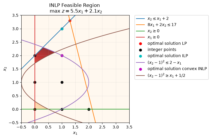
# Define the integer model
model_ncinlp = pyo.ConcreteModel(name='Simple example non-convex INP, 47-779 QuIP')
#Define the variables
model_ncinlp.x = pyo.Var([1,2], domain=pyo.Integers)
# Define the objective function
model_ncinlp.obj = pyo.Objective(rule = _obj, sense=pyo.maximize)
# Define the constraints
model_ncinlp.Constraint1 = pyo.Constraint(rule = _constraint1)

model_ncinlp.Constraint2 = pyo.Constraint(rule = _constraint2)

model_ncinlp.Constraint3 = pyo.Constraint(expr = (model_ncinlp.x[2]-1)**2 <= 2 - model_ncinlp.x[1])

model_ncinlp.Constraint4 = pyo.Constraint(expr = (model_ncinlp.x[2]-1)**2 >= 1/2 + model_ncinlp.x[1])


# Print the model
model_ncinlp.pprint()
1 Var Declarations
x : Size=2, Index={1, 2}
Key : Lower : Value : Upper : Fixed : Stale : Domain
1 : None : None : None : False : True : Integers
2 : None : None : None : False : True : Integers
1 Objective Declarations
obj : Size=1, Index=None, Active=True
Key : Active : Sense : Expression
None : True : maximize : 5.5*x[1] + 2.1*x[2]
4 Constraint Declarations
Constraint1 : Size=1, Index=None, Active=True
Key : Lower : Body : Upper : Active
None : -Inf : x[2] - (x[1] + 2) : 0.0 : True
Constraint2 : Size=1, Index=None, Active=True
Key : Lower : Body : Upper : Active
None : -Inf : 8*x[1] + 2*x[2] : 17.0 : True
Constraint3 : Size=1, Index=None, Active=True
Key : Lower : Body : Upper : Active
None : -Inf : (x[2] - 1)**2 - (2 - x[1]) : 0.0 : True
Constraint4 : Size=1, Index=None, Active=True
Key : Lower : Body : Upper : Active
None : -Inf : 0.5 + x[1] - (x[2] - 1)**2 : 0.0 : True
6 Declarations: x obj Constraint1 Constraint2 Constraint3 Constraint4
# Trying to solve the problem with BONMIN we might obtain the optimal solution, but we have no guarantees
result_obj_ncinlp = opt_bonmin.solve(model_ncinlp, tee=False)
check_solution(model_ncinlp, result_obj_ncinlp)
model_ncinlp.display()
Model 'Simple example non-convex INP, 47-779 QuIP'

  Variables:
    x : Size=2, Index={1, 2}
        Key : Lower : Value : Upper : Fixed : Stale : Domain
          1 :  None :   0.0 :  None : False : False : Integers
          2 :  None :   2.0 :  None : False : False : Integers

  Objectives:
    obj : Size=1, Index=None, Active=True
        Key  : Active : Value
        None :   True :   4.2

  Constraints:
    Constraint1 : Size=1
        Key  : Lower : Body : Upper
        None :  None :  0.0 :   0.0
    Constraint2 : Size=1
        Key  : Lower : Body : Upper
        None :  None :  4.0 :  17.0
    Constraint3 : Size=1
        Key  : Lower : Body : Upper
        None :  None : -1.0 :   0.0
    Constraint4 : Size=1
        Key  : Lower : Body : Upper
        None :  None : -0.5 :   0.0
# Define the solver COUENNE
if IN_COLAB:
    opt_couenne = pyo.SolverFactory('couenne', executable='/content/solvers/couenne')
else:
    opt_couenne = pyo.SolverFactory('couenne')
if not opt_couenne.available(exception_flag=False):
    raise RuntimeError("COUENNE not found. Run the IDAES solver setup cell near the top of this notebook.")
# Trying to solve the problem with global MINLP solver COUENNE
result_obj_ncinlp = opt_couenne.solve(model_ncinlp, tee=False)
check_solution(model_ncinlp, result_obj_ncinlp, expected_objective=4.2)
model_ncinlp.display()
Model 'Simple example non-convex INP, 47-779 QuIP'

  Variables:
    x : Size=2, Index={1, 2}
        Key : Lower : Value : Upper : Fixed : Stale : Domain
          1 :  None :   0.0 :  None : False : False : Integers
          2 :  None :   2.0 :  None : False : False : Integers

  Objectives:
    obj : Size=1, Index=None, Active=True
        Key  : Active : Value
        None :   True :   4.2

  Constraints:
    Constraint1 : Size=1
        Key  : Lower : Body : Upper
        None :  None :  0.0 :   0.0
    Constraint2 : Size=1
        Key  : Lower : Body : Upper
        None :  None :  4.0 :  17.0
    Constraint3 : Size=1
        Key  : Lower : Body : Upper
        None :  None : -1.0 :   0.0
    Constraint4 : Size=1
        Key  : Lower : Body : Upper
        None :  None : -0.5 :   0.0
ax.scatter(0,2,color='g', label='optimal solution nonconvex INLP')
ax.get_legend().remove()
ax.legend(bbox_to_anchor=(1.05, 1), loc=2, borderaxespad=0.)
fig.canvas.draw()
fig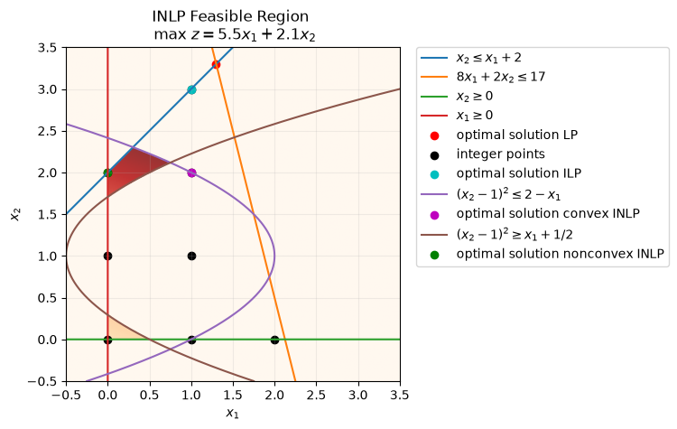
We can solve nonconvex MINLP problems, but their complexity creates substantial computational challenges.
Practice checkpoints
Use these checkpoints during the workshop to test the main ideas before moving on.
# =============================================================================
# EXERCISE 1: Change the objective sense
# =============================================================================
# Create a scratch version of the linear model that minimizes the same linear expression instead of maximizing it. Compare the new solution with the original optimum and identify which active constraints changed.
#
# Hint: Keep the feasible region unchanged so only the objective direction changes.
#
# Your code here:
# =============================================================================
Notebook Cell
# SOLUTION (hidden in workshop version):
# Scratch objective-sense check on representative feasible corner points.
candidate_points = [(0.0, 0.0), (4.0, 0.0), (0.0, 6.0), (2.0, 3.0)]
objective_values = {
    point: 5.5 * point[0] + 2.1 * point[1]
    for point in candidate_points
}
minimizer = min(objective_values, key=objective_values.get)
maximizer = max(objective_values, key=objective_values.get)
print(f"minimizer = {minimizer}; maximizer = {maximizer}")
minimizer = (0.0, 0.0); maximizer = (4.0, 0.0)
# =============================================================================
# EXERCISE 2: Add an integrality constraint
# =============================================================================
# Choose one continuous decision variable and restrict it to integer values. Re-solve the model and describe whether the objective value changes because the feasible set became smaller.
#
# Hint: Use a copied model or a fresh variable declaration so the original demonstration remains reproducible.
#
# Your code here:
# =============================================================================
Notebook Cell
# SOLUTION (hidden in workshop version):
# Compare a continuous incumbent with nearby integer candidates.
continuous_solution = (2.4, 1.6)
integer_candidates = [(2, 1), (2, 2), (3, 1), (3, 2)]
objective = lambda point: 5.5 * point[0] + 2.1 * point[1]
best_integer = max(integer_candidates, key=objective)
print(f"continuous = {continuous_solution}; best_integer = {best_integer}")
continuous = (2.4, 1.6); best_integer = (3, 2)
# =============================================================================
# EXERCISE 3: Explain a new constraint geometrically
# =============================================================================
# Add one additional linear constraint that cuts off part of the original feasible region. Sketch or describe which side of the line remains feasible and predict the effect before solving.
#
# Hint: Pick a simple bound such as a weighted sum of the two plotted variables.
#
# Your code here:
# =============================================================================
Notebook Cell
# SOLUTION (hidden in workshop version):
# Check which candidate points survive a new linear constraint.
candidate_points = [(0, 0), (4, 0), (0, 6), (2, 3), (3, 2)]
def satisfies_new_constraint(point):
    x1, x2 = point
    return x1 + x2 <= 4

remaining_points = [point for point in candidate_points if satisfies_new_constraint(point)]
print(f"remaining_feasible_points = {remaining_points}")
remaining_feasible_points = [(0, 0), (4, 0)]
Summary
In this notebook we:
Built optimization models for a production-planning example across LP, ILP, convex INLP, and nonconvex INLP forms.
Used Pyomo to declare variables, objectives, and constraints, then called solvers suited to each model class.
Compared how relaxations, integer restrictions, nonlinear constraints, and nonconvexity affect solution quality and solver behavior.
Learning objectives met: You practiced formulating optimization models, implementing them in Pyomo, choosing solver classes, and interpreting solver output across increasingly difficult model families.
Next steps: Proceed to Notebook 2: QUBO and Ising Models to learn how constrained binary models can be rewritten as unconstrained quadratic objectives.
Further reading:
David E. Bernal Neira — Davidson School of Chemical Engineering, Purdue University
Pedro Maciel Xavier — Davidson School of Chemical Engineering, Purdue University
Benjamin J. L. Murray — Davidson School of Chemical Engineering, Purdue University; Undergraduate Research Assistant
Acknowledgments
This notebook was developed by: